Importance sampling

Author: Nipun Batra

https://www.youtube.com/watch?v=TNZk8lo4e-Q&t=2733s

import numpy as np
import matplotlib.pyplot as plt
from matplotlib import rc
import seaborn as sns
import scipy.stats
%matplotlib inline

rc('font', size=16)
rc('text', usetex=True)

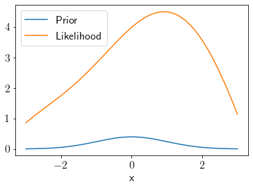
Consider the following likelihood and a Gaussian prior.

# Likelihood
def l(theta):
    return 4+ np.sin(theta) - (theta**2)/3

prior = scipy.stats.norm(0).pdf

x = np.linspace(-3, 3, 1000)

plt.plot(x, prior(x),label='Prior')
plt.plot(x, l(x),label='Likelihood')
plt.legend();
plt.xlabel('x');

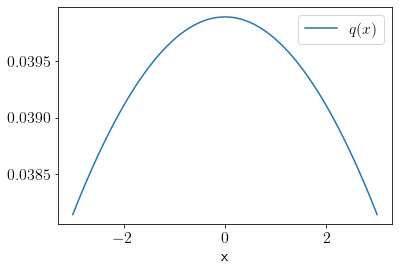
We define a sampling distribution \(q(x)\) as the following.

q_rvs = scipy.stats.norm(loc=0, scale=10)
q = q_rvs.pdf

plt.plot(x, q(x), label='$q(x)$');
plt.xlabel('x');
plt.legend();

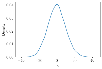
Let’s draw a large number of samples from \(q(x)\) distribution.

q_samples = q_rvs.rvs(size=10000)

sns.kdeplot(q_samples);
plt.xlabel('x');

We can find the marginal likelihood \(z\) using the following technique.

(1)\[\begin{align} z &= \int likelihood(x)\cdot prior(x)\cdot dx\\ z &= \int \frac{likelihood(x)\cdot prior(x)}{q(x)}\cdot q(x) \cdot dx\\ z &= \int w(x) \cdot q(x) \cdot dx\\ z &\approx \frac{1}{N}\sum\limits_{i=1}^{N}w(x) \end{align}\]

prior_eval_q = prior(q_samples)
likelihood_eval_q = l(q_samples)
z = (prior_eval_q*likelihood_eval_q/q_samples).mean()
z

-0.508527841674989

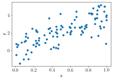
Importance sampling for linear regression

Likelihood for linear regression can be given as the following,

\(p(\mathbf{y}|\theta) \sim \mathcal{N}(\theta \mathbf{x}, \sigma_n^2I)\)

theta_gt = 4
sigma_n = 1

# generate some samples

x = np.random.uniform(0, 1, size = 100)
y = np.random.normal(theta_gt*x, sigma_n)

plt.scatter(x, y);
plt.xlabel('x');plt.ylabel('y');

We will use the following \(q\) distribution in this problem.

# Proposal

q_rvs = scipy.stats.norm(loc=3, scale=10)
q = q_rvs.pdf

Prior on \(\theta\) is Standard Gaussian distribution.

prior = scipy.stats.norm(0).pdf

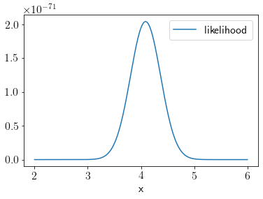
Likelihood is given as the following,

# Likelihood
def l(theta):
    return scipy.stats.multivariate_normal.pdf(y, mean=theta*x, cov=3*np.eye(len(x)))

xu = np.linspace(2, 6, 1000)
k = []
for xt in xu:
    k.append(l(xt))
plt.plot(xu, k, label='likelihood');
plt.xlabel('x');
plt.legend();

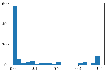
plt.hist(scipy.stats.norm(10*x, 1).pdf(y), density=False, bins=20);

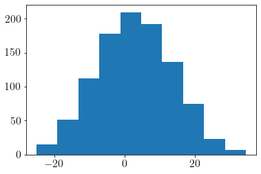
Let us draw a few samples from the \(q\) distribution.

n_samples = 1000
q_samples = q_rvs.rvs(size=n_samples)

We calculate the \(w(x)\) using the samples drawn from the \(q\) distribution.

plt.hist(q_samples)

w = np.zeros(n_samples)
for i in range(n_samples):
    theta_i = q_samples[i]
    likelihood_i = l(theta_i)
    prior_i = prior(theta_i)
    q_i = q_rvs.pdf(theta_i)
    w_i = likelihood_i*prior_i/q_i
    w[i] = w_i

It is easy to retrive marginal likelihood now.

marginal_likelihood = np.mean(w)

Let us compute the full posterior distribution.

post = np.zeros(n_samples)
for i in range(n_samples):
    theta_i = q_samples[i]
    likelihood_i = l(theta_i)
    prior_i = prior(theta_i)
    post_i = likelihood_i*prior_i
    post[i] = post_i/marginal_likelihood

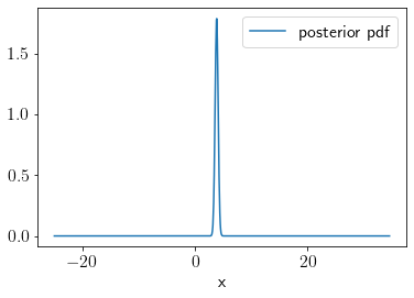
We can visualize the posterior distribution as the following,

idx = np.argsort(q_samples)
plt.plot(q_samples[idx], post[idx], label='posterior pdf');
plt.xlabel('x')
plt.legend()

print('approx posterior mean', np.mean(q_samples[np.where(post>1.25)]))

approx posterior mean 3.7819254239877527