Local Lengthscale GP with PyMC¶

In this chapter, we explore a non-stationary GP discussed by [PKB08] with PyMC.

import numpy as np
import matplotlib.pyplot as plt
from matplotlib import rc
import pymc3 as pm
from sklearn.cluster import KMeans
import warnings
from multiprocessing import Pool
warnings.filterwarnings('ignore')

rc('font', size=16)

Let us define both stationary and non-statioanry RBF kernels,

### Stationary GP
def kernel(a, b, lenghtscale, std):
    """
    Borrowed from Nando De Freita's lecture code
    https://www.cs.ubc.ca/~nando/540-2013/lectures/gp.py
    """
    sqdist = np.square(a - b.T)
    return std**2*np.exp(-.5 * (1/lenghtscale) * sqdist)

### LLS GP
def global_kernel(x1, x2, l1, l2, std):
    sqdist = np.square(x1 - x2.T)
    l1l2meansqr = (np.square(l1)[:, np.newaxis, :] + np.square(l2)[np.newaxis, :, :]).squeeze()/2
#     print(sqdist.shape, l1l2meansqr.shape)
    return std**2 * pm.math.matrix_dot(np.sqrt(l1),np.sqrt(l2.T)) * (1/np.sqrt(l1l2meansqr)) * np.exp(-sqdist/l1l2meansqr)

def local_kernel(x1, x2, lengthscale):
    """
    Borrowed from Nando De Freita's lecture code
    https://www.cs.ubc.ca/~nando/540-2013/lectures/gp.py
    """
    sqdist = np.square(x1 - x2.T)
    return np.exp(-.5 * (1/lengthscale) * sqdist)

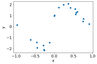
We will test the efficacy of these models on a step function data.

n_train = 21
np.random.seed(1234)

# Generate data
def f(X):  # target function
    return np.sin(5*X) + np.sign(X)

X = np.random.uniform(-1, 1, (n_train, 1)).reshape(-1,1)  # data
Y = f(X)[:, 0] + np.random.normal(0,0.2,n_train)
plt.scatter(X, Y);
plt.xlabel('x');
plt.ylabel('y');

../../_images/2021-03-17-lls-gp-pymc3_6_0.png

Stationary GP model¶

basic_model = pm.Model()

with basic_model:

    # Priors for unknown model parameters
    # Variance
    kernel_std = pm.Lognormal("kernel_std", 0, 0.1)
    # Length scale
    kernel_ls = pm.Lognormal("kernel_ls", 0, 1)
    noise_sigma = pm.Lognormal("noise_sigma", 0, 1)
    K = kernel(X, X, kernel_ls, kernel_std) 
    K += np.eye(X.shape[0]) * np.power(noise_sigma, 2)
    
    y = pm.MvNormal("y", mu = 0, cov = K, observed = Y.squeeze())

pm.model_to_graphviz(basic_model.model)

../../_images/2021-03-17-lls-gp-pymc3_9_0.svg

Let us find MAP estimate of paramaters.

map_estimate = pm.find_MAP(model=basic_model)
map_estimate

100.00% [17/17 00:00<00:00 logp = -17.781, ||grad|| = 3.4567]

{'kernel_std_log__': array(0.02655438),
 'kernel_ls_log__': array(-2.68569403),
 'noise_sigma_log__': array(-1.27853804),
 'kernel_std': array(1.02691009),
 'kernel_ls': array(0.06817386),
 'noise_sigma': array(0.27844408)}

Now, we will sample from the posterior.

with basic_model:
    # draw 2000 posterior samples per chain
    trace = pm.sample(2000,return_inferencedata=False,tune=2000)

Auto-assigning NUTS sampler...
Initializing NUTS using jitter+adapt_diag...
Multiprocess sampling (4 chains in 4 jobs)
NUTS: [noise_sigma, kernel_ls, kernel_std]

100.00% [16000/16000 00:15<00:00 Sampling 4 chains, 0 divergences]

Sampling 4 chains for 2_000 tune and 2_000 draw iterations (8_000 + 8_000 draws total) took 15 seconds.

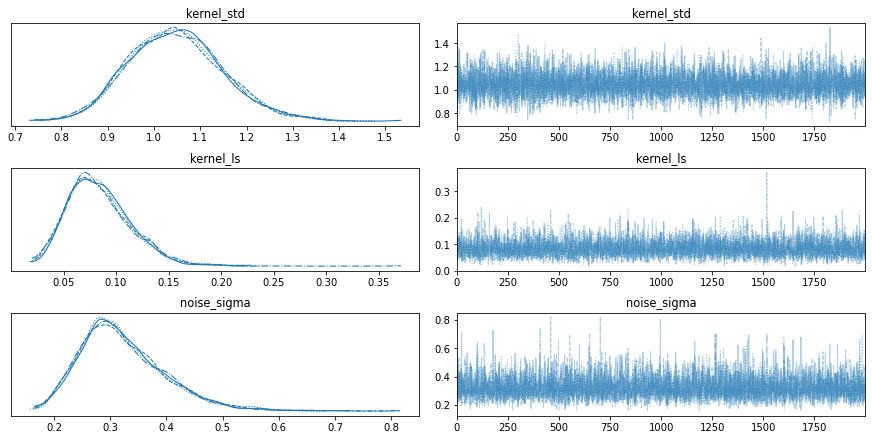
import arviz as az

az.plot_trace(trace);

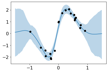
../../_images/2021-03-17-lls-gp-pymc3_14_0.png

Now, we will infer the \(y\) values at new input locations.

test_x = np.linspace(-1.5, 1.5, 100).reshape(-1, 1)
train_x = X
train_y = Y

def post(train_x, train_y, test_x, kernel, kernel_ls, kernel_std, noise):
    N = len(train_x)
    K = kernel(train_x, train_x, kernel_ls, kernel_std)+noise**2*np.eye(len(train_x))
    N_star = len(test_x)
    K_star = kernel(train_x,  test_x, kernel_ls, kernel_std)
    K_star_star = kernel(test_x, test_x, kernel_ls, kernel_std)
    posterior_mu = K_star.T@np.linalg.inv(K)@(train_y)
    posterior_sigma = K_star_star - K_star.T@np.linalg.inv(K)@K_star
    
    # Instead of size = 1, we can also sample multiple times given a single length scale, kernel_std and noise
    return np.random.multivariate_normal(posterior_mu, posterior_sigma, size=1)

# Make predictions at new locations.
train_y = Y.squeeze()
n_samples = 500
preds = np.stack([post(train_x, train_y, test_x=test_x, kernel=kernel, kernel_ls=trace['kernel_ls'][b],
                             kernel_std=trace['kernel_std'][b],
                             noise=trace['noise_sigma'][b])
                  for b in range(n_samples)])

ci = 95
ci_lower = (100 - ci) / 2
ci_upper = (100 + ci) / 2
preds_mean = preds.reshape(n_samples, len(test_x)).mean(0)
preds_lower = np.percentile(preds, ci_lower, axis=0)
preds_upper = np.percentile(preds, ci_upper, axis=0)

plt.plot(test_x,preds.reshape(n_samples, len(test_x)).mean(axis=0))

plt.scatter(train_x, train_y, c='black', zorder=3, label='data')
plt.fill_between(test_x.flatten(), preds_upper.flatten(), preds_lower.flatten(), alpha=.3, label='95% CI');

LLS GP¶

We will learn local lengthscales at 3 input locations choosen by KMeans clustering.

n_local = 3
lls_model = pm.Model()
param_X = KMeans(n_local, random_state=0).fit(X).cluster_centers_

with lls_model:
    
    ### Local GP
    # local lengthscale
    local_ls = pm.Lognormal("local_ls", 0, 1)
    param_ls = pm.Lognormal("param_ls", 0, 1, shape=(n_local, 1))
    local_K = local_kernel(param_X, param_X, local_ls)
    local_K_star = local_kernel(X, param_X, local_ls)
    
    ### global GP
    # global lengthscales
    global_ls = pm.math.exp(pm.math.matrix_dot(local_K_star, pm.math.matrix_inverse(local_K), pm.math.log(param_ls)))
    # global variance
    global_std = pm.Lognormal("global_std", 0, 1)
    # global noise
    global_noise_sigma = pm.Lognormal("global_noise_sigma", 0, 1)
    
    global_K = global_kernel(X, X, global_ls, global_ls, global_std)
    global_K += np.eye(X.shape[0])*global_noise_sigma**2
    
    y = pm.MvNormal("y", mu = 0, cov = global_K, observed = Y)

pm.model_to_graphviz(lls_model.model)

../../_images/2021-03-17-lls-gp-pymc3_22_0.svg

Let us find MAP estimate of paramaters.

NSmap_estimate = pm.find_MAP(model=lls_model)
NSmap_estimate

100.00% [18/18 00:00<00:00 logp = -16.642, ||grad|| = 0.93967]

{'local_ls_log__': array(-0.88024402),
 'param_ls_log__': array([[-0.28197464],
        [-0.05336731],
        [-1.54950142]]),
 'global_std_log__': array(0.09507128),
 'global_noise_sigma_log__': array(-1.61986434),
 'local_ls': array(0.41468171),
 'param_ls': array([[0.75429281],
        [0.94803173],
        [0.21235382]]),
 'global_std': array(1.09973724),
 'global_noise_sigma': array(0.19792555)}

with lls_model:
    # draw 2000 posterior samples per chain
    trace = pm.sample(4000,return_inferencedata=False,tune=2000)

Auto-assigning NUTS sampler...
Initializing NUTS using jitter+adapt_diag...
Multiprocess sampling (4 chains in 4 jobs)
NUTS: [global_noise_sigma, global_std, param_ls, local_ls]

100.00% [24000/24000 00:42<00:00 Sampling 4 chains, 57 divergences]

Sampling 4 chains for 2_000 tune and 4_000 draw iterations (8_000 + 16_000 draws total) took 43 seconds.
There were 12 divergences after tuning. Increase `target_accept` or reparameterize.
There were 13 divergences after tuning. Increase `target_accept` or reparameterize.
There were 18 divergences after tuning. Increase `target_accept` or reparameterize.
There were 14 divergences after tuning. Increase `target_accept` or reparameterize.

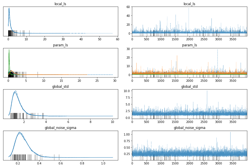
import arviz as az
with lls_model:
    az.plot_trace(trace);

../../_images/2021-03-17-lls-gp-pymc3_26_0.png

Let us predict the values at new locations.

test_x = np.linspace(-1.5, 1.5, 100).reshape(-1, 1)
train_x = X
train_y = Y

def post(local_ls, param_ls, global_std, global_noise):
    N = len(train_x)
    param_K_inv = np.linalg.inv(local_kernel(param_X, param_X, local_ls))
    local_K = local_kernel(train_x, param_X, local_ls)
    global_ls = np.exp(local_K@param_K_inv@param_ls)
    local_K_star = local_kernel(test_x, param_X, local_ls)
    global_ls_star = np.exp(local_K_star@param_K_inv@param_ls)
    K = global_kernel(train_x, train_x, global_ls, global_ls, global_std)+np.eye(N)*global_noise**2
    K_inv = pm.math.matrix_inverse(K)
    K_star = global_kernel(train_x, test_x, global_ls, global_ls_star, global_std)
    posterior_mu = pm.math.matrix_dot(K_star.T,K_inv,train_y)
    
    return posterior_mu.eval()
    # Instead of size = 1, we can also sample multiple times given a single length scale, kernel_std and noise
    return np.random.multivariate_normal(posterior_mu.eval(), posterior_sigma.eval(), size=1)

# Make predictions at new locations.
n_samples = 100

preds = np.stack([post(local_ls=trace['local_ls'][b],
                       param_ls=trace['param_ls'][b],
                       global_std=trace['global_std'][b],
                      global_noise=trace['global_noise_sigma'][b])
                  for b in range(n_samples)])

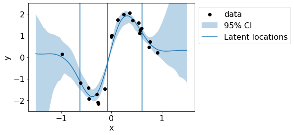
Let us visualize predictive mean and variance.

ci = 95
ci_lower = (100 - ci) / 2
ci_upper = (100 + ci) / 2
preds_mean = preds.reshape(n_samples, len(test_x)).mean(0)
preds_lower = np.percentile(preds, ci_lower, axis=0)
preds_upper = np.percentile(preds, ci_upper, axis=0)

plt.plot(test_x,preds.reshape(n_samples, len(test_x)).mean(axis=0))

plt.scatter(train_x, train_y, c='black', zorder=3, label='data')
plt.fill_between(test_x.flatten(), preds_upper.flatten(), preds_lower.flatten(), alpha=.3, label='95% CI');
for x_loc in param_X:
    plt.vlines(x_loc, -3, 3);
plt.vlines(x_loc, -3, 3, label='Latent locations');
plt.legend(bbox_to_anchor=(1,1));
plt.ylim(-2.5,2.5);
plt.xlabel('x')
plt.ylabel('y');

../../_images/2021-03-17-lls-gp-pymc3_32_0.png

Let us visualize the latent lengthscales.

local_ls = NSmap_estimate['local_ls']
param_ls = NSmap_estimate['param_ls']
local_K = local_kernel(param_X, param_X, local_ls)
local_K_star = local_kernel(test_x, param_X, local_ls)

global_ls = pm.math.exp(pm.math.matrix_dot(local_K_star, pm.math.matrix_inverse(local_K), pm.math.log(param_ls)))
plt.plot(test_x, global_ls.eval(), label='Local lengthscales', color='r');
plt.vlines(param_X.squeeze(), *plt.ylim(), label='latent locations')
plt.xlabel('x')
plt.ylabel('lengthscales');
plt.legend(bbox_to_anchor=(1,1));

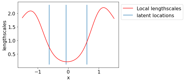
../../_images/2021-03-17-lls-gp-pymc3_34_0.png

We see that lengthscales are low in the center region where the underlying function is having a sudden jump. Thus, LLS model is giving us sensible predictions.

Prog-ML

Local Lengthscale GP with PyMC

Contents

Local Lengthscale GP with PyMC¶

Stationary GP model¶

LLS GP¶