HMM Simulation for Unfair Casino Problem#
A programming introduction to HMMs for unfair casino problem
toc: true
badges: true
comments: true
author: Nipun Batra
categories: [ML]
In this notebook we shall create a Hidden Markov Model [1] for the Unfair Casino problem [2]. In short the problem is as follows: In a casino there may be two die- one fair and the other biased. The biased die is much more likely to produce a 6 than the other numbers. With the fair die all the outcomes (1 through 6) are equally likely. For the biased die, probability of observing a 6 is 0.5 and observing 1,2,3,4,5 is 0.1 each. Also, there are probabilies associated with the choice of a die to be thrown. The observer is only able to observe the values of die being thrown, without having a knowldge whether a fair or biased die were used.
In all it matches the description of a discrete Hidden Markov Model. The different components of the Discrete HMM are as follows:
Observed States : 1 through 6 on the die faces
Hidden States : Fair or Biased Die
Prior (pi) : Probability that the first throw is made from a fair or a biased die, which is : Pr (first throw is fair) and Pr (first throw is biased), which is represented as a 1 X 2 row matrix
Transition Matrix (A): Matrix encoding the probability of the 4 possible transition between fair and biased die, which are: Fair-> Fair, Fair-> Biased, Biased-> Fair and Biased->Biased, which is represented as a 2 X 2 matrix
Emission Matrix (B) : Matrix encoding the probability of an observation given the hidden state. It is a 2 X 6 Matrix
Next, we import the basic set of libraries used for matrix manipulation and for plotting.
import numpy as np
import matplotlib.pyplot as plt
import matplotlib
#Setting Font Size as 20
matplotlib.rcParams.update({'font.size': 20})
Next, we define the different components of HMM which were described above.
'''
Pi : Fair die is twice as likely as biased die

A  : The die thrower likes to keep in one state (fair/biased), and the tranisition from
1. Fair-> Fair : .95
2. Fair->Biased: 1-.95=.05
3. Biased->Biased: .90
4. Biased->Biased=1-.90=.10

B  : The fair die is equally likely to produce observations 1 through 6, for the biased die
Pr(6)=0.5 and Pr(1)=Pr(2)=Pr(3)=Pr(4)=Pr(5)=0.1
'''
pi=np.array([2.0/3,1.0/3])
A=np.array([[.95,.05],[.1,.9]])
B=np.array([[1.0/6 for i in range(6)],[.1,.1,.1,.1,.1,.5]])
Now based on these probability sequences we need to produce a sequence of observed and hidden states. We use the notion of weighted sampling, which basically means that terms/states with higher probabilies assigned to them are more likely to be selected/sampled. For example,let us consider the starting state. For this we need to use the pi matrix, since that encodes the likiliness of starting in a particular state. We observe that for starting in Fair state the probability is .667 and twice that of starting in Biased state. Thus, it is much more likely that we start in Fair state. We use Fitness Proportionate Selection [3] to sample states based on weights (probability). For selection of starting state we would proceed as follows:
We choose a random value between 0 and 1
We iterate over the list of values (prior) and iteratively subtract the value at current position from the number which we chose at random and as soon as it becomes negative, we return the index. Let us demonstrate this with a function.
'''
Returns next state according to weigted probability array. Code based on Weighted random generation in Python [4]
'''
def next_state(weights):
    choice = random.random() * sum(weights)
    for i, w in enumerate(weights):
        choice -= w
        if choice < 0:
            return i
We test the above function by making a call to it 1000 times and then we try to see how many times do we get a 0 (Fair) wrt 1 (Biased), given the pi vector.
count=0
for i in range(1000):
    count+=next_state(pi)
print "Expected number of Fair states:",1000-count
print "Expected number of Biased states:",count
Expected number of Fair states: 649
Expected number of Biased states: 351
Thus, we can see that we get approximately twice the number of Fair states as Biased states which is as expected.
Next, we write the following functions:
create_hidden_sequence (pi,A,length): which creates a hidden sequence (Markov Chain) of desired length based on Pi and A. The algorithm followed is as follows: We choose the first state as described above. Next on the basis of current state, we see it’s transition matrix and assign the next state by weighted sampling (by invoking next_state with argument as A[current_state])
create_observed_sequence (hidden_sequence,B): which create an observed sequence based on hidden states and associated B. Based on current hidden state, we use it’s emission parameters to sample the observation.
def create_hidden_sequence(pi,A,length):
    out=[None]*length
    out[0]=next_state(pi)
    for i in range(1,length):
        out[i]=next_state(A[out[i-1]])
    return out

def create_observation_sequence(hidden_sequence,B):
    length=len(hidden_sequence)
    out=[None]*length
    for i in range(length):
        out[i]=next_state(B[hidden_sequence[i]])
    return out
Thus, using these functions and the HMM paramters we decided earlier, we create length 1000 sequence for hidden and observed states.
hidden=np.array(create_hidden_sequence(pi,A,1000))
observed=np.array(create_observation_sequence(hidden,B))
'''Group all contiguous values in tuple. Recipe picked from Stack Overflow [5]'''
def group(L):
    first = last = L[0]
    for n in L[1:]:
        if n - 1 == last: # Part of the group, bump the end
            last = n
        else: # Not part of the group, yield current group and start a new
            yield first, last
            first = last = n
    yield first, last # Yield the last group

'''Create tuples of the form (start, number_of_continuous values'''
def create_tuple(x):
    return [(a,b-a+1) for (a,b) in x]
#Tuples of form index value, number of continuous values corresponding to Fair State
indices_hidden_fair=np.where(hidden==0)[0]
tuples_contiguous_values_fair=list(group(indices_hidden_fair))
tuples_start_break_fair=create_tuple(tuples_contiguous_values_fair)

#Tuples of form index value, number of continuous values corresponding to Biased State
indices_hidden_biased=np.where(hidden==1)[0]
tuples_contiguous_values_biased=list(group(indices_hidden_biased))
tuples_start_break_biased=create_tuple(tuples_contiguous_values_biased)

#Tuples for observations
observation_tuples=[]
for i in range(6):
    observation_tuples.append(create_tuple(group(list(np.where(observed==i)[0]))))
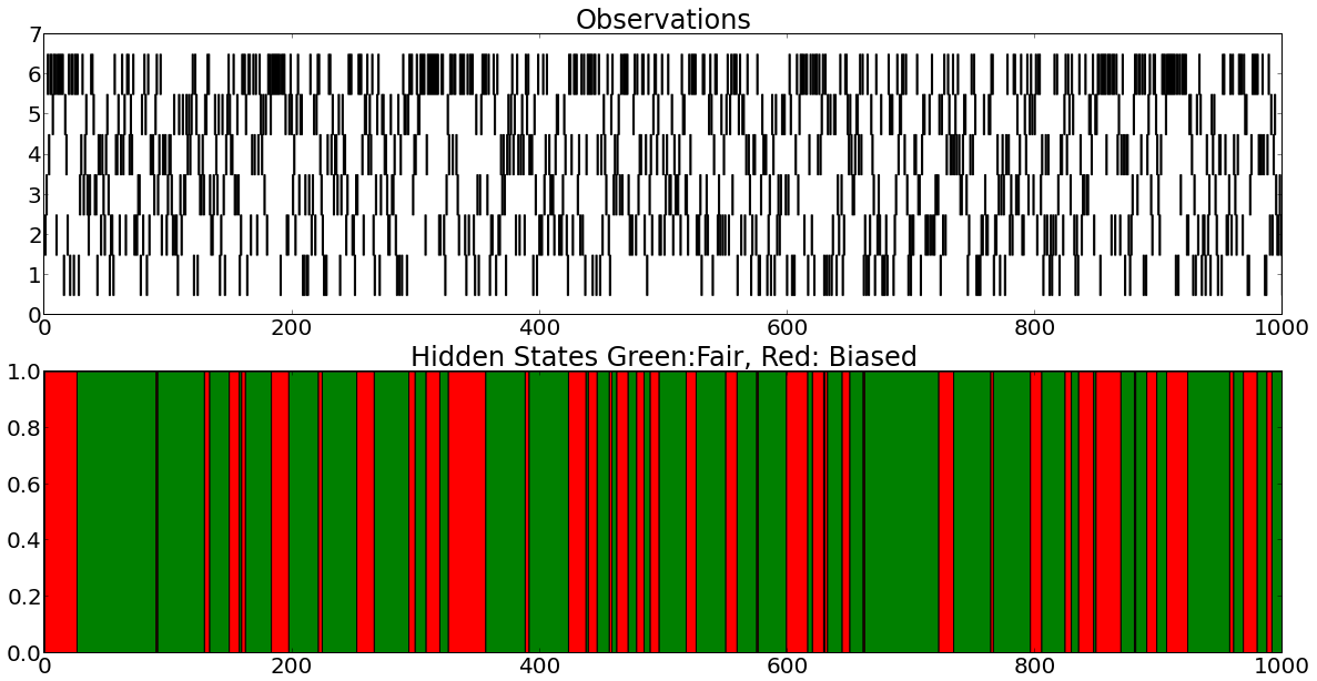
Now we plot the hidden and observation sequences
plt.figsize(20,10)
plt.subplot(2,1,1)
plt.xlim((0,1000));
plt.title('Observations');
for i in range(6):
    plt.broken_barh(observation_tuples[i],(i+0.5,1),facecolor='k');
plt.subplot(2,1,2);
plt.xlim((0,1000));
plt.title('Hidden States Green:Fair, Red: Biased');
plt.broken_barh(tuples_start_break_fair,(0,1),facecolor='g');
plt.broken_barh(tuples_start_break_biased,(0,1),facecolor='r');