Bayesian model selection¶

Author: Zeel B Patel

http://mlg.eng.cam.ac.uk/teaching/4f13/1920/bayesian finite regression.pdf (Last slide) http://mlg.eng.cam.ac.uk/teaching/4f13/1920/marginal likelihood.pdf

import numpy as np
import scipy.stats
import matplotlib.pyplot as plt
from matplotlib import rc
rc('font', size=14)
from scipy.optimize import minimize
import warnings
warnings.filterwarnings('ignore')
from time import time

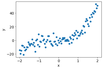
Pseudo-random data (degree 3 polynomial)¶

np.random.seed(0)

N = 100
sigma_n = 5 # noise in data
sigma_w = 100 # parameter variance

x = np.linspace(-2,2,N).reshape(-1,1)
f_x = 4*x**3 + 3*x**2 + 2*x + 1
epsilon = np.random.normal(loc=0, scale=sigma_n, size=N).reshape(-1,1)
y = f_x + epsilon

plt.scatter(x, y);
plt.xlabel('x');plt.ylabel('y');

../../_images/2021-03-29-bayesian-model-selection_4_0.png

Marginal likelihood pdf¶

def LogMarginalLikelihoodPdf(x, y):
    return np.log(scipy.stats.multivariate_normal.pdf(y.squeeze(), np.zeros(N), (x@x.T)*sigma_w**2 + np.eye(N)*sigma_n**2))

Models¶

x_M0 = x.copy()
x_M1 = np.hstack([np.ones((N,1)), x])
x_M2 = np.hstack([np.ones((N,1)), x, x**2])
x_M3 = np.hstack([np.ones((N,1)), x, x**2, x**3])
x_M4 = np.hstack([np.ones((N,1)), x, x**2, x**3, x**4])
x_M5 = np.hstack([np.ones((N,1)), x, x**2, x**3, x**4, x**5])
x_M6 = np.hstack([np.ones((N,1)), x, x**2, x**3, x**4, x**5, x**6])
x_M7 = np.hstack([np.ones((N,1)), x, x**2, x**3, x**4, x**5, x**6, x**7])

Model selection¶

scores = [LogMarginalLikelihoodPdf(x_M, y) for x_M in [x_M0, x_M1, x_M2, x_M3, x_M4, x_M5, x_M6, x_M7]]
plt.plot(scores);
plt.xlabel('Degree of polynomial');
plt.ylabel('Log Marginal Likelihood \n(Higher is better)');
plt.xticks(range(len(scores)));

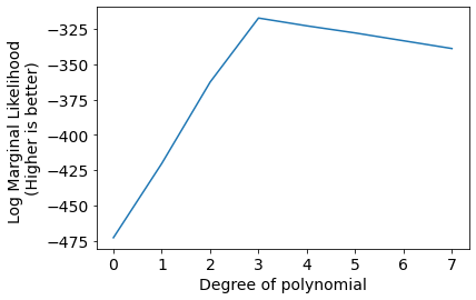
We can infer that Degree 3 polynomial is best suited to model current data.

Model selection with parameter optimization¶

def NegLogMarginalLikelihoodPdf(params, x, y): # Negative log marginal likelihood (written in GP fashion)
    sigma_n, sigma_w = params
    K = (x@x.T)*sigma_w**2 + np.eye(N)*sigma_n**2
    K_inv = np.linalg.pinv(K)
    nll = 0.5*y.T@K_inv@y + 0.5*np.log(np.linalg.det(K)) + (len(y)/2)*np.log(2*np.pi)
    return nll[0,0]

Negscores = []
sig_n_list = []
sig_w_list = []
sig_w = 10
sig_n = 10
for i, x_M in enumerate([x_M0, x_M1, x_M2, x_M3, x_M4, x_M5, x_M6, x_M7]):
    init = time()
    result = minimize(fun=NegLogMarginalLikelihoodPdf, x0=(sig_n, sig_w), args=(x_M, y))
    sig_n_opt, sig_w_opt = result.x
    sig_n_list.append(sig_n_opt)
    sig_w_list.append(sig_w_opt)
    print(f'degree = {i}, sigma_w={sig_w_opt}, sig_n_opt={sig_n_opt}', 'time:',time()-init,'seconds')
    Negscores.append(NegLogMarginalLikelihoodPdf((sig_n_opt, sig_w_opt), x_M, y))
plt.plot(Negscores);
plt.xlabel('Degree of polynomial');
plt.ylabel('Neg Log Marginal Likelihood \n(Lower is better)');
plt.xticks(range(len(Negscores)));

degree = 0, sigma_w=11.386419730789676, sig_n_opt=10.409619988275981 time: 0.16215753555297852 seconds
degree = 1, sigma_w=8.895627576152828, sig_n_opt=8.940430356187846 time: 0.08962178230285645 seconds
degree = 2, sigma_w=7.119736606266272, sig_n_opt=6.9430152775634495 time: 0.14646410942077637 seconds
degree = 3, sigma_w=3.219312493175096, sig_n_opt=4.710523287770871 time: 0.14163684844970703 seconds
degree = 4, sigma_w=2.6041389205399996, sig_n_opt=4.739086634960693 time: 0.2660367488861084 seconds
degree = 5, sigma_w=-2.5131468222243427, sig_n_opt=4.745522282327305 time: 0.17346620559692383 seconds
degree = 6, sigma_w=2.163988485988779, sig_n_opt=4.768321344889457 time: 0.5917925834655762 seconds
degree = 7, sigma_w=1.6084504892174767, sig_n_opt=4.758818020810231 time: 0.32204294204711914 seconds

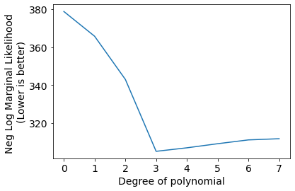
../../_images/2021-03-29-bayesian-model-selection_14_1.png

We can see the best set of hyper-parameters selected by gradient descent on negative log likelihood for indivisual models (degree of polynomial).

Drawbacks¶

This method does not scale well with big data (while doing parameter optimization), because of matrix inversion.
- Potential solution: optimize parameters with chepaer methods, then use Marginal likelihood for model selection

Using empirical bayes (Bishop)¶

http://krasserm.github.io/2019/02/23/bayesian-linear-regression/

alpha = 1/sigma_w**2
beta = 1/sigma_n**2

Marginal likelihood pdf¶

def posterior(Phi, t, alpha, beta, return_inverse=False):
    """Computes mean and covariance matrix of the posterior distribution."""
    S_N_inv = alpha * np.eye(Phi.shape[1]) + beta * Phi.T.dot(Phi)
    S_N = np.linalg.inv(S_N_inv)
    m_N = beta * S_N.dot(Phi.T).dot(t)

    if return_inverse:
        return m_N, S_N, S_N_inv
    else:
        return m_N, S_N

def log_marginal_likelihood(Phi, t, alpha, beta):
    """Computes the log of the marginal likelihood."""
    N, M = Phi.shape

    m_N, _, S_N_inv = posterior(Phi, t, alpha, beta, return_inverse=True)
    
    E_D = beta * np.sum((t - Phi.dot(m_N)) ** 2)
    E_W = alpha * np.sum(m_N ** 2)
    
    score = M * np.log(alpha) + \
            N * np.log(beta) - \
            E_D - \
            E_W - \
            np.log(np.linalg.det(S_N_inv)) - \
            N * np.log(2 * np.pi)

    return 0.5 * score

Bscores = [log_marginal_likelihood(x_M, y, alpha, beta) for x_M in [x_M0, x_M1, x_M2, x_M3, x_M4, x_M5, x_M6, x_M7]]
plt.plot(Bscores);
plt.xlabel('Degree of polynomial');
plt.ylabel('Log Marginal Likelihood \n(Higher is better)');
plt.xticks(range(len(Bscores)));

../../_images/2021-03-29-bayesian-model-selection_21_0.png

Results are exactly the same as the previous method.

Paramater tuning¶

def fit(Phi, t, alpha_0=1e-5, beta_0=1e-5, max_iter=200, rtol=1e-5, verbose=False):
    """
    Jointly infers the posterior sufficient statistics and optimal values 
    for alpha and beta by maximizing the log marginal likelihood.
    
    Args:
        Phi: Design matrix (N x M).
        t: Target value array (N x 1).
        alpha_0: Initial value for alpha.
        beta_0: Initial value for beta.
        max_iter: Maximum number of iterations.
        rtol: Convergence criterion.
        
    Returns:
        alpha, beta, posterior mean, posterior covariance.
    """
    
    N, M = Phi.shape

    eigenvalues_0 = np.linalg.eigvalsh(Phi.T.dot(Phi))

    beta = beta_0
    alpha = alpha_0

    for i in range(max_iter):
        beta_prev = beta
        alpha_prev = alpha

        eigenvalues = eigenvalues_0 * beta

        m_N, S_N, S_N_inv = posterior(Phi, t, alpha, beta, return_inverse=True)

        gamma = np.sum(eigenvalues / (eigenvalues + alpha))
        alpha = gamma / np.sum(m_N ** 2)

        beta_inv = 1 / (N - gamma) * np.sum((t - Phi.dot(m_N)) ** 2)
        beta = 1 / beta_inv

        if np.isclose(alpha_prev, alpha, rtol=rtol) and np.isclose(beta_prev, beta, rtol=rtol):
            if verbose:
                print(f'Convergence after {i + 1} iterations.')
            return alpha, beta, m_N, S_N

    if verbose:
        print(f'Stopped after {max_iter} iterations.')
    return alpha, beta, m_N, S_N

for i, x_M in enumerate([x_M0, x_M1, x_M2, x_M3, x_M4, x_M5, x_M6, x_M7]):
    init = time()
    alpha, beta, m_N, S_N = fit(x_M, y, rtol=1e-5, verbose=True)
    print('Degree',i,'sigma_w',1/np.sqrt(alpha),'sigma_n', 1/np.sqrt(beta))
    print('Degree',i,'sigma_w',sig_w_list[i],'sigma_n', sig_n_list[i], '(Earlier method)')
    print('time:',time()-init,'seconds')

Convergence after 3 iterations.
Degree 0 sigma_w 11.386046324847063 sigma_n 10.409625056741909
Degree 0 sigma_w 11.386419730789676 sigma_n 10.409619988275981 (Earlier method)
time: 0.0020685195922851562 seconds
Convergence after 3 iterations.
Degree 1 sigma_w 8.89562357924776 sigma_n 8.940424942304906
Degree 1 sigma_w 8.895627576152828 sigma_n 8.940430356187846 (Earlier method)
time: 0.006841897964477539 seconds
Convergence after 3 iterations.
Degree 2 sigma_w 7.119729723394079 sigma_n 6.943013815169844
Degree 2 sigma_w 7.119736606266272 sigma_n 6.9430152775634495 (Earlier method)
time: 0.0012140274047851562 seconds
Convergence after 4 iterations.
Degree 3 sigma_w 3.219311433389237 sigma_n 4.710523173354075
Degree 3 sigma_w 3.219312493175096 sigma_n 4.710523287770871 (Earlier method)
time: 0.0022554397583007812 seconds
Convergence after 6 iterations.
Degree 4 sigma_w 2.6041361190065677 sigma_n 4.739086719922639
Degree 4 sigma_w 2.6041389205399996 sigma_n 4.739086634960693 (Earlier method)
time: 0.0025718212127685547 seconds
Convergence after 9 iterations.
Degree 5 sigma_w 2.5131492993598394 sigma_n 4.745518078421809
Degree 5 sigma_w -2.5131468222243427 sigma_n 4.745522282327305 (Earlier method)
time: 0.003193378448486328 seconds
Convergence after 9 iterations.
Degree 6 sigma_w 2.1639963673023725 sigma_n 4.768325837603502
Degree 6 sigma_w 2.163988485988779 sigma_n 4.768321344889457 (Earlier method)
time: 0.0029621124267578125 seconds
Convergence after 6 iterations.
Degree 7 sigma_w 1.6084472283522588 sigma_n 4.758819295283589
Degree 7 sigma_w 1.6084504892174767 sigma_n 4.758818020810231 (Earlier method)
time: 0.002556324005126953 seconds

This method is extremely fast than the previous method. We get close answers while using any of the two methods.

Prog-ML

Bayesian model selection

Contents

Bayesian model selection¶

Pseudo-random data (degree 3 polynomial)¶

Marginal likelihood pdf¶

Models¶

Model selection¶

Model selection with parameter optimization¶

Drawbacks¶

Using empirical bayes (Bishop)¶

Marginal likelihood pdf¶

Paramater tuning¶