Deep Kernel Learning¶

We now briefly discuss deep kernel learning. Quoting the deep kernel learning paper: scalable deep kernels combine the structural properties of deep learning architectures with the non-parametric flexibility of kernel methods.

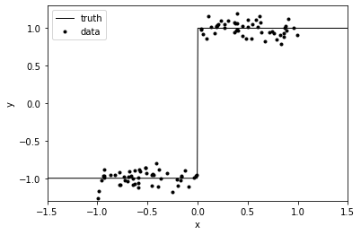
We will transform our input via a neural network and feed the transformed input to our GP. To illustrate, we will create a simple step function dataset (heavily inspired from this excellent writeup on tinyGP). We will be comparing our deep kernel with the RBF kernel.

import torch
import torch.nn as nn
import torch.nn.functional as F
import matplotlib.pyplot as plt 
import seaborn as sns
from mpl_toolkits.axes_grid1 import make_axes_locatable

import pyro.contrib.gp as gp
import pyro

torch.manual_seed(0)

noise = 0.1

x = torch.sort(torch.distributions.Uniform(low=-1., high=1.).sample([100, 1]), 0)[0]
x_squeeze = x.squeeze()
y = 2 * (x_squeeze > 0) - 1 + torch.distributions.Normal(loc=0.0, scale=noise).sample([len(x)])
t =torch.linspace(-1.5, 1.5, 500)

plt.plot(t, 2 * (t > 0) - 1, "k", lw=1, label="truth")
plt.plot(x_squeeze, y, ".k", label="data")
plt.xlim(-1.5, 1.5)
plt.ylim(-1.3, 1.3)
plt.xlabel("x")
plt.ylabel("y")
_ = plt.legend()

class Net(nn.Module):
    def __init__(self):
        super().__init__()
        self.fc1 = nn.Linear(1, 5)
        self.fc2 = nn.Linear(5, 5)
        self.fc3 = nn.Linear(5, 2)

    def forward(self, x):
        x = F.relu(self.fc1(x))
        x = F.relu(self.fc2(x))
        x = self.fc3(x)
        return x

pyro.clear_param_store()
n = Net()
# Using a separate lengthscale for each dimension
rbf = gp.kernels.RBF(input_dim=2, lengthscale=torch.ones(2))
deep_kernel = gp.kernels.Warping(rbf, iwarping_fn=n)
likelihood = gp.likelihoods.Gaussian()
model_deep = gp.models.VariationalGP(
    X=x,
    y=y,
    kernel=deep_kernel,
    likelihood=likelihood,
    whiten=True,
    jitter=2e-3,
)

model_rbf = gp.models.VariationalGP(
    X=x,
    y=y,
    kernel=gp.kernels.RBF(input_dim=1),
    likelihood=likelihood,
    whiten=True,
    jitter=2e-3,
)

As we can see, it is fairly straightforward to create a deep kernel by combining a regular kernel with a neural network. We can also confirm our deep kernel by printing it below. It should also be noted that unlike our earlier code, we explicitly specified lengthscale in our above example to be a vector of two values. This will allow our model to learn a different lengthscale for each dimension.

deep_kernel

Warping(
  (kern): RBF()
  (iwarping_fn): Net(
    (fc1): Linear(in_features=1, out_features=5, bias=True)
    (fc2): Linear(in_features=5, out_features=5, bias=True)
    (fc3): Linear(in_features=5, out_features=2, bias=True)
  )
)

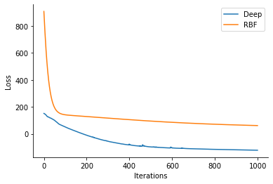
losses_deep = gp.util.train(model_deep, num_steps=1000)
losses_rbf = gp.util.train(model_rbf, num_steps=1000)
plt.plot(losses_deep, label='Deep')
plt.plot(losses_rbf, label='RBF')
sns.despine()
plt.legend()
plt.xlabel("Iterations")
plt.ylabel("Loss")

Text(0, 0.5, 'Loss')

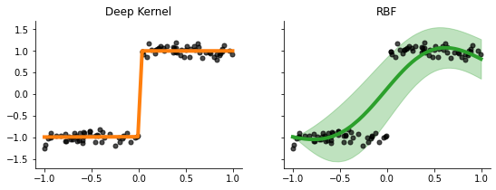
with torch.no_grad():
    fig, ax = plt.subplots(ncols=2, sharey=True, figsize=(9, 3))
    for i, (model_name, model) in enumerate(zip(["Deep Kernel", "RBF"], [model_deep, model_rbf])):
        mean, var = model(x)
        ax[i].plot(x.squeeze(), mean, lw=4, color=f'C{i+1}', label=model_name)
        ax[i].fill_between(x_squeeze, mean-torch.sqrt(var), mean+torch.sqrt(var), alpha=0.3, color=f'C{i+1}')
        ax[i].scatter(x.squeeze(), y, color='k', alpha=0.7, s=25)
        ax[i].set_title(model_name)
sns.despine()

with torch.no_grad():
    z = n(x)
    plt.plot(x.squeeze(), z, label='Transformed Input')
    plt.scatter(x.squeeze(), y, color='k', alpha=0.7, s=25, label='Data')
    plt.legend()

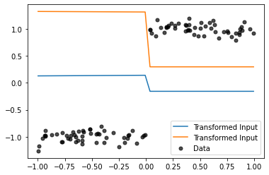
Our deep kernel transform the data into a step function like data, thus, making it better suited in comparison to the RBF kernel, which has a hard time owing to the sudden jump around x=0.0.

rbf.lengthscale

tensor([0.7100, 0.3202], grad_fn=<AddBackward0>)

Finally, we can confirm from the above code that we learn a different lengthscale corresponding to the two dimensions (transformation of the 1 dimensional data by the neural network).

Prog-ML

Deep Kernel Learning

Deep Kernel Learning¶