Automatic relevance determination (ARD)¶

Author: Zeel B Patel

import scipy.stats
import GPy
from scipy.optimize import minimize
import numpy as np
import matplotlib.pyplot as plt
from matplotlib import rc
import warnings
warnings.filterwarnings('ignore')
%matplotlib inline

rc('text', usetex=True)
rc('font', size=16)

To understand the concept of ARD, let us generate a symthetic dataset where all features are not equally important.

np.random.seed(0)
N = 400
X = np.empty((N, 3))
y = np.empty((N, 1))

cov = [[1,0,0,0.99],[0,1,0,0.6],[0,0,1,0.1],[0.99,0.6,0.1,1]]

samples = np.random.multivariate_normal(np.zeros(4), cov, size=N)

X[:,:] = samples[:,:3]
y[:,:] = samples[:,3:4]
print('Correlation between X1 and y', np.corrcoef(X[:,0], y.ravel())[1,0])
print('Correlation between X2 and y', np.corrcoef(X[:,1], y.ravel())[1,0])
print('Correlation between X3 and y', np.corrcoef(X[:,2], y.ravel())[1,0])

Correlation between X1 and y 0.7424364387053712
Correlation between X2 and y 0.4771760788020134
Correlation between X3 and y 0.07463999808005005

Let us fit a GP model with a common lengthscale for all features.

model = GPy.models.GPRegression(X, y, GPy.kern.RBF(input_dim=3, ARD=False))
model.optimize()
model

Model: GP regression
Objective: 346.85990977337315
Number of Parameters: 3
Number of Optimization Parameters: 3
Updates: True

GP_regression.	value	constraints
rbf.variance	111.47290536431103	+ve
rbf.lengthscale	26.862865061479035	+ve
Gaussian_noise.variance	0.3083839240873474	+ve

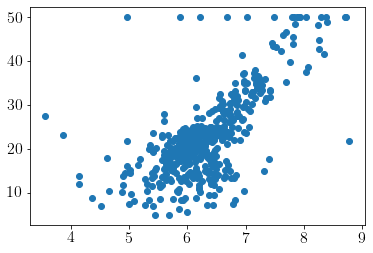
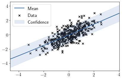
Visualizing fit over \(X_1\)

model.plot(visible_dims=[0]);

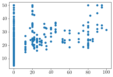
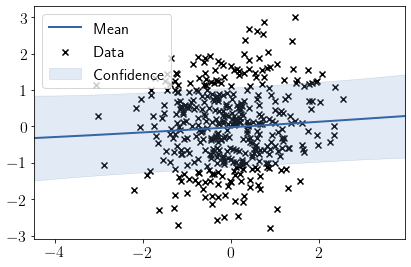
Visualizing fit over \(X_3\)

model.plot(visible_dims=[2]);

Now, let us turn on the ARD and see the values of lengthscales learnt.

model = GPy.models.GPRegression(X, y, GPy.kern.RBF(input_dim=3, ARD=True))
model.optimize()
model.kern.lengthscale

We can see that the lengthscale for \(X_3\) is abnormally larger than the other two due to lowest correlation with data.

Real-data¶

Let us try a real dataset and see what insights we can get by ARD experiment on it.

from sklearn.datasets import load_boston

X, y = load_boston(return_X_y=True)
y = y.reshape(-1,1)
X.shape, y.shape

((506, 13), (506, 1))

Let us see what do we get from ARD enabled GP fit.

model = GPy.models.GPRegression(X, y, GPy.kern.RBF(input_dim=13, ARD=True))
model.optimize()
model.kern.lengthscale

index	GP_regression.rbf.lengthscale	constraints
[0]	22.24437029	+ve
[1]	33.16175836	+ve
[2]	143.39745522	+ve

We can see some features seem more important (e.g. [5],[7]) and others do not. Let us verify this visually.

plt.scatter(X[:,5], y);

../../_images/2021-04-16-ard-gp_20_0.png

plt.scatter(X[:,1], y);

../../_images/2021-04-16-ard-gp_21_0.png

We can see a strong patern in [5] but we can not see any patterns in [1].

index	GP_regression.rbf.lengthscale	constraints
[0]	288.47316598	+ve
[1]	1958.66785662	+ve
[2]	96.63008923	+ve
[3]	522.58028671	+ve
[4]	262.09440505	+ve
[5]	3.15337665	+ve
[6]	267.59752767	+ve
[7]	2.07260971	+ve
[8]	154.25307337	+ve
[9]	218.28124322	+ve
[10]	48.57585913	+ve
[11]	282.84461914	+ve
[12]	22.50407090	+ve

Prog-ML

Automatic relevance determination (ARD)

Contents

Automatic relevance determination (ARD)¶

Real-data¶