GP v/s Deep GP on 2d data¶

In this notebook, we will be comparing three models (all RBF kernel) on a simulated 2d data:

GP
GP with ARD
Deep GP

import GPy

import numpy as np
import pyDOE2
from sklearn.metrics import mean_squared_error
# Plotting tools
from matplotlib import pyplot as plt
from matplotlib import rc

rc('font', size=16)
rc('text', usetex=True)

import warnings
warnings.filterwarnings('ignore')

# GPy: Gaussian processes library
import GPy

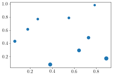
We generate pseudo data using the following function,

\[ y = \frac{(x_1+2)(2-x_2^2)}{3} \]

np.random.seed(0)
X = pyDOE2.doe_lhs.lhs(2, 9, random_state=0)
func = lambda x: ((x[:, 0]+2)*(2-x[:, 1])**2)/3
y = func(X)

plt.scatter(X[:,0], X[:, 1],s=y*50);

../../_images/2021-04-16-GP-vs-DeepGP_6_0.png

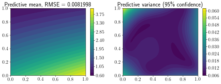
GP without ARD¶

k_2d = GPy.kern.RBF(input_dim=2, lengthscale=1)

m = GPy.models.GPRegression(X, y.reshape(-1, 1), k_2d)
m.optimize();

Model: GP regression
Objective: -5.479737333080651
Number of Parameters: 3
Number of Optimization Parameters: 3
Updates: True

GP_regression.	value	constraints
rbf.variance	72.28075242747792	+ve
rbf.lengthscale	3.382677032484262	+ve
Gaussian_noise.variance	9.922601887760885e-06	+ve

x_1 = np.linspace(0, 1, 40)
x_2 = np.linspace(0, 1, 40)

X1, X2 = np.meshgrid(x_1, x_2)
X_new = np.array([(x1, x2) for x1, x2 in zip(X1.ravel(), X2.ravel())])
Y_true = func(X_new)

Y_pred, Y_cov = m.predict(X_new)
Y_95 = 2*np.sqrt(Y_cov)

fig, ax = plt.subplots(1,2,figsize=(12,4))
mp = ax[0].contourf(X1, X2, Y_pred.reshape(*X1.shape), levels=30)
fig.colorbar(mp, ax=ax[0])
ax[0].set_title(f'Predictive mean, RMSE = {mean_squared_error(Y_true, Y_pred, squared=False).round(7)}');

mp = ax[1].contourf(X1, X2, Y_95.reshape(*X1.shape), levels=30)
ax[1].set_title(f'Predictive variance (95\% confidence)')
fig.colorbar(mp, ax=ax[1]);

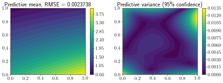
../../_images/2021-04-16-GP-vs-DeepGP_13_0.png

GP with ARD¶

k_2d_ARD = GPy.kern.RBF(input_dim=2, lengthscale=1, ARD=True)

m = GPy.models.GPRegression(X, y.reshape(-1, 1), k_2d_ARD)
m.optimize();

Model: GP regression
Objective: -6.917350273214053
Number of Parameters: 4
Number of Optimization Parameters: 4
Updates: True

GP_regression.	value	constraints
rbf.variance	40.53729208947549	+ve
rbf.lengthscale	(2,)	+ve
Gaussian_noise.variance	4.3169473160951275e-29	+ve

Y_pred, Y_cov = m.predict(X_new)
Y_95 = 2*np.sqrt(Y_cov)

fig, ax = plt.subplots(1,2,figsize=(12,4))
mp = ax[0].contourf(X1, X2, Y_pred.reshape(*X1.shape), levels=30)
fig.colorbar(mp, ax=ax[0])
ax[0].set_title(f'Predictive mean, RMSE = {mean_squared_error(Y_true, Y_pred, squared=False).round(7)}');

mp = ax[1].contourf(X1, X2, Y_95.reshape(*X1.shape), levels=30)
ax[1].set_title(f'Predictive variance (95\% confidence)')
fig.colorbar(mp, ax=ax[1]);

../../_images/2021-04-16-GP-vs-DeepGP_19_0.png

m.parameters[0].lengthscale

We see that lengthscale for \(x_1\) is higher because of linear relationship with the output and lengthscale for \(x_2\) is higher due to quadratic relationship with the output.

Deep GP¶

import deepgp
layers = [1, 1,  X.shape[1]]
inits = ['PCA']*(len(layers)-1)
kernels = []
for i in layers[1:]:
    kernels += [GPy.kern.RBF(i, ARD=True)]
    
m = deepgp.models.DeepGP(layers,Y=y.reshape(-1, 1), X=X, 
                  inits=inits, 
                  kernels=kernels, # the kernels for each layer
                  num_inducing=4, back_constraint=False)

m.optimize()

Model: deepgp
Objective: 10.244507717038887
Number of Parameters: 45
Number of Optimization Parameters: 45
Updates: True

index	GP_regression.rbf.lengthscale	constraints	priors
[0]	5.80242511	+ve
[1]	1.80657554	+ve

deepgp.	value	constraints
obslayer.inducing inputs	(4, 1)
obslayer.rbf.variance	23.808937388338997	+ve
obslayer.rbf.lengthscale	4.451925378737478	+ve
obslayer.Gaussian_noise.variance	0.0020011072507906376	+ve
obslayer.Kuu_var	(4,)	+ve
obslayer.latent space.mean	(9, 1)
obslayer.latent space.variance	(9, 1)	+ve
layer_1.inducing inputs	(4, 2)
layer_1.rbf.variance	30.67508979761088	+ve
layer_1.rbf.lengthscale	(2,)	+ve
layer_1.Gaussian_noise.variance	0.0012460891277525125	+ve
layer_1.Kuu_var	(4,)	+ve

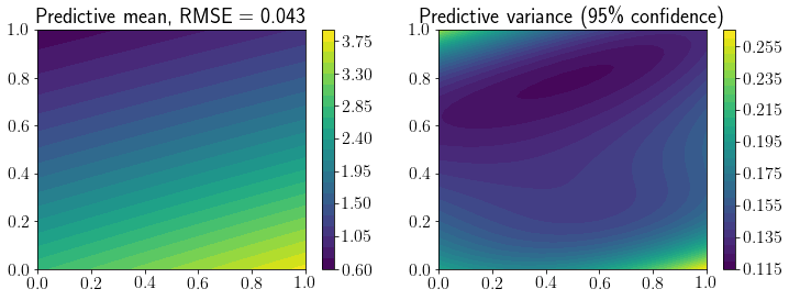
Y_pred, Y_cov = m.predict(X_new)
Y_95 = 2*np.sqrt(Y_cov)

fig, ax = plt.subplots(1,2,figsize=(12,4))
mp = ax[0].contourf(X1, X2, Y_pred.reshape(*X1.shape), levels=30)
fig.colorbar(mp, ax=ax[0])
ax[0].set_title(f'Predictive mean, RMSE = {mean_squared_error(Y_true, Y_pred, squared=False).round(3)}');

mp = ax[1].contourf(X1, X2, Y_95.reshape(*X1.shape), levels=30)
ax[1].set_title(f'Predictive variance (95\% confidence)')
fig.colorbar(mp, ax=ax[1]);

../../_images/2021-04-16-GP-vs-DeepGP_27_0.png

Not working Pinball_plot : https://github.com/lawrennd/talks/blob/gh-pages/deepgp_tutorial.py

Prog-ML

GP v/s Deep GP on 2d data

Contents

GP v/s Deep GP on 2d data¶

GP without ARD¶

GP with ARD¶

Deep GP¶