
Bayesian linear regression#
Author: Nipun Batra
import numpy as np
import matplotlib.pyplot as plt
from matplotlib import rc
import seaborn as sns
import pymc3 as pm
import arviz as az

rc('font', size=16)
rc('text', usetex=True)
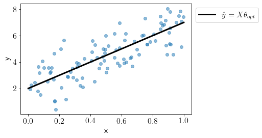
Let us generate data from known parameters.
theta_gt = [2, 5]
X = np.random.uniform(0, 1, 100)
Y = theta_gt[0] + theta_gt[1] * X + np.random.normal(0, 1, 100)
We can see the optimal fit on this data.
plt.scatter(X, Y, alpha=0.5)
x_line = np.linspace(0, 1, 1000)
y_line_gt = theta_gt[0] + theta_gt[1] * x_line
plt.plot(x_line, y_line_gt, color='k',lw=3, label='$\hat{y} = X\\theta_{opt}$');
plt.xlabel('x');
plt.ylabel('y');
plt.legend(bbox_to_anchor=(1,1));
We can define Bayesian linear regression model in PyMC as the following,
basic_model = pm.Model()

with basic_model:

    # Priors for unknown model parameters
    theta = pm.Normal("theta", mu=0, sigma=10, shape=2)
    sigma = pm.HalfNormal("sigma", sigma=1)
    X_ = pm.Data('features', X)
    # Expected value of outcome
    mu = theta[0] + theta[1] * X_

    # Likelihood (sampling distribution) of observations
    Y_obs = pm.Normal("Y_obs", mu=mu, sigma=sigma, observed=Y)
Let us get the MAP for model paramaters.
map_estimate = pm.find_MAP(model=basic_model)
map_estimate
{'theta': array([2.06886375, 4.76338553]),
 'sigma_log__': array(0.0340025),
 'sigma': array(1.03458719)}
Let us draw a large number of samples from the posterior.
with basic_model:
    # draw 500 posterior samples
    trace = pm.sample(2000,return_inferencedata=False,tune=1000)
Auto-assigning NUTS sampler...
Initializing NUTS using jitter+adapt_diag...
Multiprocess sampling (4 chains in 4 jobs)
NUTS: [sigma, theta]
Sampling 4 chains for 1_000 tune and 2_000 draw iterations (4_000 + 8_000 draws total) took 5 seconds.
We can visualize the posterior distributions over individual paramaters as the following,
az.plot_trace(trace);
/home/patel_zeel/anaconda3/lib/python3.8/site-packages/arviz/data/io_pymc3.py:96: FutureWarning: Using `from_pymc3` without the model will be deprecated in a future release. Not using the model will return less accurate and less useful results. Make sure you use the model argument or call from_pymc3 within a model context.
  warnings.warn(
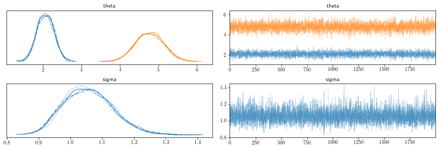
Below is the summary statistics of the posterior.
with basic_model:
    display(az.summary(trace, round_to=2))
| mean | sd | hdi_3% | hdi_97% | mcse_mean | mcse_sd | ess_bulk | ess_tail | r_hat | |
|---|---|---|---|---|---|---|---|---|---|
| theta[0] | 2.06 | 0.22 | 1.65 | 2.47 | 0.00 | 0.0 | 3486.19 | 3563.27 | 1.0 |
| theta[1] | 4.77 | 0.37 | 4.09 | 5.48 | 0.01 | 0.0 | 3587.88 | 3968.01 | 1.0 |
| sigma | 1.06 | 0.08 | 0.92 | 1.21 | 0.00 | 0.0 | 4405.63 | 3833.57 | 1.0 |
Let us predict at the new input locations. This would mean to sample from the likelihood using posterior parameters.
x_new = np.linspace(-1, 1, 100) # 50 input values between -3 and 3
with basic_model:
    pm.set_data({'features': x_new})
    posterior = pm.sample_posterior_predictive(trace)

preds = posterior['Y_obs']
preds.shape
(8000, 100)
y_mean = np.mean(preds, axis=0)
y_std = np.std(preds, axis=0)

plt.scatter(X, Y, c='k', zorder=10, label='Data',alpha=0.2)
plt.plot(x_new, y_mean, label='Prediction Mean',color='black',lw=2)
plt.fill_between(x_new, y_mean - 2*y_std, y_mean + 2*y_std, alpha=0.12, label='Uncertainty Interval ($\mu\pm2\sigma$)',color='violet')
plt.xlabel('$x$')
plt.ylabel('$y$')
plt.ylim(-14, 16)
plt.legend(loc='lower right');
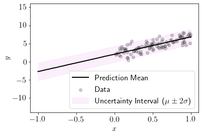
We can see that uncertainty is covering 95% of the samples here and hence model is giving sensible estimate of uncertainty.
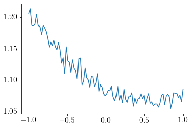
We can see that uncertainty is lower in the region where the dataset is lying.
plt.plot(x_new, y_std);
Laplacian Prior (LASSO)#
Let us use a Laplacial prior instead of Gaussian. Note that this settings matches with Lasso regression.
class Lasso:
    def __init__(self, b):
        self.b = b

    def fit(self, X, y):
        lasso_model = pm.Model()
        self.model = lasso_model
        with self.model:

            # Priors for unknown model parameters
            theta = pm.Laplace("theta", mu=0, b=self.b, shape=2)
            sigma = pm.HalfNormal("sigma", sigma=1)
            X_ = pm.Data('features', X)
            # Expected value of outcome
            mu = theta[0] + theta[1] * X_

            # Likelihood (sampling distribution) of observations
            Y_obs = pm.Normal("Y_obs", mu=mu, sigma=sigma, observed=Y)
            trace_lasso = pm.sample(1500,return_inferencedata=False,tune=500)
        self.model = lasso_model
        self.trace = trace_lasso

    def plot(self):
        az.plot_trace(self.trace)

    def predict(self, X):
        with self.model:
            pm.set_data({'features': X})
            posterior = pm.sample_posterior_predictive(self.trace)
        self.posterior = posterior
Let us draw posterior with different initial prior paramaters.
import logging
logger = logging.getLogger('pymc3')
logger.setLevel(logging.ERROR)

out = {}
regs = {}
for b in [0.02, 0.05, 0.07, 0.1, 0.2, 1]:
    print('b',b)
    reg = Lasso(b)
    reg.fit(X, Y)
    regs[b] = reg
    out[b] = reg.trace['theta']
b 0.02
b 0.05
b 0.07
b 0.1
b 0.2
b 1
Let us visualize the posterior distribution over theta.
fig, ax = plt.subplots(ncols=2)
for i, b in enumerate([0.02, 0.05, 0.07, 0.1, 0.2, 1]):
    sns.kdeplot(out[b][:, 0], ax=ax[0], label=b)
    sns.kdeplot(out[b][:, 1], ax=ax[1], label=b)
plt.legend();
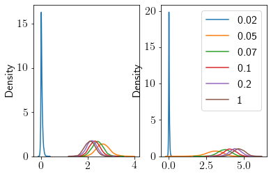
Higher values of \(b\) seem to give close to the original predictions.
We define a custom function to visualize the posterior fit on the new input locations by varying initial paramaters of prior.
def plot_custom(b):
    reg = regs[b]
    reg.predict(x_new)
    preds = reg.posterior['Y_obs']
    y_mean = np.mean(preds, axis=0)
    y_std = np.std(preds, axis=0)
    plt.scatter(X, Y, c='k', zorder=10, label='Data',alpha=0.2)
    plt.plot(x_new, y_mean, label='Prediction Mean',color='black',lw=2)
    plt.fill_between(x_new, y_mean - 2*y_std, y_mean + 2*y_std, alpha=0.12, label='Uncertainty Interval ($\mu\pm2\sigma$)',color='violet')
    plt.xlabel('$x$')
    plt.ylabel('$y$')
    plt.ylim(-14, 16)
    plt.legend(loc='upper left')
plot_custom(0.02)
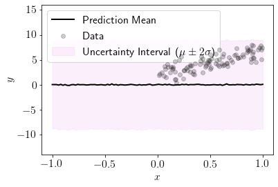
plot_custom(0.05)
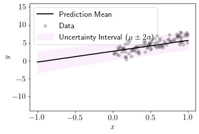
We can see that for \(b=0.05\) model is giving sensible predictions.