Stationarity of stochastic processes II¶

https://bookdown.org/gary_a_napier/time_series_lecture_notes/ChapterThree.html

import numpy as np
import matplotlib.pyplot as plt
from matplotlib import rc
from matplotlib.animation import FuncAnimation

rc('font', size=16)
rc('text', usetex=True)
rc('animation', html='jshtml')

The function below generates multiple samples of $n$ length, $d$ order stationary process using the following AR equation (AR stands for auto-regressive),

y_{t} = \sum_{i = 1}^{d} y_{t - d} ϕ_{t - d} + N (0, 1)

def AR(phi, n):
    order = len(phi)
    x = [0 for _ in range(order)]
    for i in range(n-order):
        tmp = np.sum(np.array(x[-order:])*phi+np.random.normal(0,1))
        x.append(tmp)
    return x

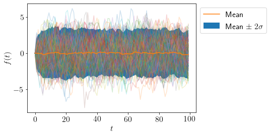
Let us visualize many samples from AR( $d = 1, n = 100, ϕ = {0.8}$ ) stochastic process.

def plot_AR(Phi, n):
    X = []
    for i in range(201):
        X.append(AR(Phi, n))
    for sample in X:
        plt.plot(sample, alpha=0.2);

    means = np.mean(X, axis=0)
    std2 = np.std(X, axis=0)*2
    plt.plot(means, label='Mean')
    plt.fill_between(range(n), means-std2, means+std2, label='Mean $\pm\;2\sigma$');
    plt.legend(bbox_to_anchor=(1,1));
    plt.xlabel('$t$')
    plt.ylabel('$f(t)$')

plot_AR([0.8], 100)

../../_images/2021-03-23-Stationarity-stochastic-processes_7_0.png

Let us try changing $ϕ = {- 0.8}$

plot_AR([-0.8], 100)

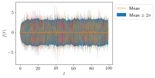
../../_images/2021-03-23-Stationarity-stochastic-processes_9_0.png

We can see that mean and variance of samples at any time $t$ is almost constant.

Let us draw some samples from a AR( $d = 1, n = 100, ϕ = {1.01}$ ).

plot_AR([1.01], 100)

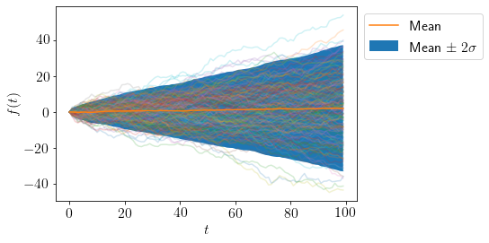
../../_images/2021-03-23-Stationarity-stochastic-processes_11_0.png

We can see that mean is almost constant over time but variance is varying significantly.

What are the insights? For AR(1) process,

(41)¶

\begin{aligned} y_{t} & = y_{t - 1} ϕ_{t - 1} + Z_{t}, Z_{t} \sim N (0, 1) \\ y_{t} - y_{t - 1} ϕ_{t - 1} & = Z_{t} \\ (1 - B ϕ_{t - 1}) y_{t} & = Z_{t} \end{aligned}

We define charesterstic equation as following,

f_{c} (B) = 1 - B ϕ_{t - 1} = 0

If roots (magnitude of roots in case of imaginary roots) of $f_{c} (B)$ are outside unit circle or in other words, $| B | > 1$ , AR(1) process is stationary.

For $ϕ = 0.8$ , $B = 1.25$ so, AR( $d = 1, ϕ = 0.8$ ) is a stationary process.
For $ϕ = 1.01$ , $B = 0.99$ so, AR( $d = 1, ϕ = 1.01$ ) is a non-stationary process.

Same rule is applicable for AR( $d$ ) process for any value of $d$ .

Let us try an AR( $d = 3$ ) process now.

We take AR( $d = 3, n = 100, ϕ = {0.1, 0.2, 0.3}$ ).

plot_AR([0.1, 0.2, 0.3], 100)

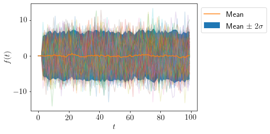
../../_images/2021-03-23-Stationarity-stochastic-processes_14_0.png

From the graph, process looks stationary, let us find the roots of the following charesterstic equation,

f_{c} (B) = 1 - 0.1 B - 0.2 B^{2} - 0.3 B^{3} = 0

np.roots([-0.3, -0.2, -0.1, 1]), np.abs(np.roots([-0.3, -0.2, -0.1, 1]))

(array([-0.95244656+1.3359895j, -0.95244656-1.3359895j,
         1.23822645+0.j       ]),
 array([1.64073837, 1.64073837, 1.23822645]))

We see that all the roots are outside the unit circle, so the process must be stationary.

Let us try one more example.

AR( $d = 3, n = 10, ϕ = {0.6, 0.8, 0.9}$ )

plot_AR([0.6, 0.8, 0.9], 10)

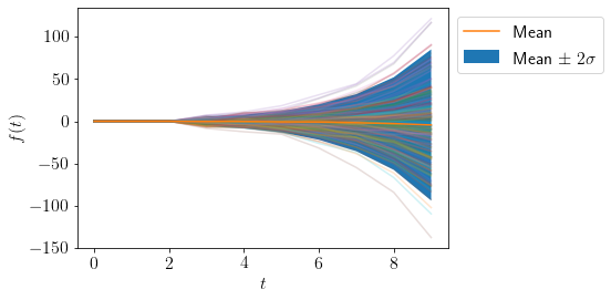
../../_images/2021-03-23-Stationarity-stochastic-processes_18_0.png

np.roots([-0.9, -0.8, -0.6, 1]), np.abs(np.roots([-0.9, -0.8, -0.6, 1]))

(array([-0.77387424+1.04284911j, -0.77387424-1.04284911j,
         0.6588596 +0.j        ]),
 array([1.29862066, 1.29862066, 0.6588596 ]))

We can see that atleast one root is inside the unit circle, thus the process is non-stationary.

Prog-ML

Stationarity of stochastic processes II

Stationarity of stochastic processes II¶