Eigen values¶

In this notebook, we will look at eigen values. https://youtu.be/PFDu9oVAE-g

import numpy as np
import matplotlib.pyplot as plt
from matplotlib import rc
from matplotlib.animation import FuncAnimation

rc('font', size=16)
rc('text', usetex=True)
rc('animation', html='jshtml')

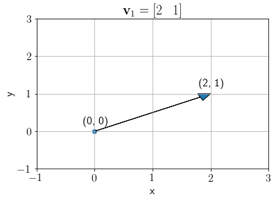
Consider a vector \(\mathbf{v}_1\) below,

\[\begin{split} \mathbf{v}_1 = \begin{bmatrix} 2 & 1\\ \end{bmatrix} \end{split}\]

v1 = np.array([2, 1])

plt.arrow(x=0, y=0, dx=v1[0], dy=v1[1], shape='full', head_width=0.2, head_length=0.2, length_includes_head=True)
plt.text(0-0.2, 0+0.2, f'({0}, {0})')
plt.text(v1[0]-0.2, v1[1]+0.2, f'({v1[0]}, {v1[1]})')
plt.scatter(0, 0)
plt.grid()
plt.ylim((-1, 3))
plt.xlim(-1, 3);
plt.xlabel('x');plt.ylabel('y');
plt.title('$\mathbf{v}_1 = [2\;\;\;1]$');

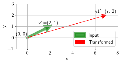
\(\mathbf{v}_1\) gets transformed to \(\mathbf{v}_1'\) after applying a transformation \(A\).

\[ \mathbf{v}_1' = A\mathbf{v}_1 \]

We define a useful function for plotting a linear transformation on any vector.

def plot_transformation(x, A, ax, annotate=False):
    arrow_in = ax.arrow(x=0, y=0, dx=x[0, 0], dy=x[1, 0], shape='full', head_width=0.4, 
                         head_length=0.4, color='green', lw=8, alpha=0.6, length_includes_head=True)
    ax.grid()
    
    # Applying transformation
    Ax = A@x
    
    # Get current min, max
    ymin, ymax = (min(Ax[1], x[1], 0)-1, max(Ax[1], x[1], 0)+1)
    xmin, xmax = (min(Ax[0], x[0], 0)-1, max(Ax[0], x[0], 0)+1)
    
    # Check and update according to previous
    ax.set_ylim(min(ymin, ax.set_ylim()[0]), max(ymax, ax.set_ylim()[1]))
    ax.set_xlim(min(xmin, ax.set_xlim()[0]), max(xmax, ax.set_xlim()[1]))
    
    arrow_out = ax.arrow(x=0, y=0, dx=Ax[0, 0], dy=Ax[1, 0], shape='full', head_width=0.4, 
                          head_length=0.4, color='red', length_includes_head=True)
    if annotate:
        ax.text(0-1, 0+0.2, f'({0}, {0})')
        ax.text(x[0, 0]-1, x[1, 0]+0.2, f'v1=({x[0, 0]}, {x[1, 0]})')
        ax.text(Ax[0, 0]-1, Ax[1, 0]+0.2, f'v1\'=({Ax[0, 0]}, {Ax[1, 0]})')
    ax.legend([arrow_in, arrow_out, ], ['Input','Transformed',], loc='lower right')
    ax.set_aspect('equal')
    ax.set_xlabel('x');ax.set_ylabel('y')

We plot the following transformation.

\[\begin{split} A = \begin{bmatrix} 3 & 1\\ 0 & 2 \end{bmatrix} \mathbf{v}_1 = \begin{bmatrix} 2\\ 1\\ \end{bmatrix} \end{split}\]

\[ \mathbf{v}_1' = A\mathbf{v}_1 \]

fig, ax = plt.subplots()
plot_transformation(np.array([2, 1]).reshape(-1, 1), np.array([[3, 1], [0, 2]]), ax, annotate=True);

Now, we define a function to subtract a scaler \(\lambda\) from diagonal of \(A\).

def A_minus_lmd(A, lmd):
    A[0, 0] = A[0, 0] - lmd
    A[1, 1] = A[1, 1] - lmd
    return A

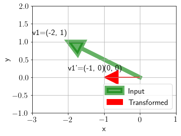
Transforming a random vector with \(A-\boldsymbol{\lambda} I\) matrix.

fig, ax = plt.subplots()
plot_transformation(np.array([-2, 1]).reshape(-1,1), A_minus_lmd(np.array([[3, 1], [0, 2]]), 2), ax, annotate=True);

Let us visualize many such random vectors after transforming with \(A - \boldsymbol{\lambda} I\) (taking \(\boldsymbol{\lambda} = 2\)).

lmd = 2
fig, ax = plt.subplots()

def update(x):
    i, j = x
    ax.cla()
    plot_transformation(np.array([-i, j]).reshape(-1,1), A_minus_lmd(np.array([[3, 1], [0, 2]]), lmd), ax)
    ax.set_xlim(-11,11)
    ax.set_ylim(-11,11)

frames = []
for i in range(-5, 5, 1):
    for j in range(-5, 5, 1):
        frames.append((i, j))

plt.tight_layout()
anim = FuncAnimation(fig, update, frames)
plt.close()
anim

Now we visualize these random vectors after transforming with \(A - \boldsymbol{\lambda} I\) (taking \(\boldsymbol{\lambda} = 3\)).

lmd = 3
fig, ax = plt.subplots()

def update(x):
    i, j = x
    ax.cla()
    plot_transformation(np.array([-i, j]).reshape(-1,1), A_minus_lmd(np.array([[3, 1], [0, 2]]), lmd), ax)
    ax.set_xlim(-11,11)
    ax.set_ylim(-11,11)

frames = []
for i in range(-5, 5, 1):
    for j in range(-5, 5, 1):
        frames.append((i, j))

plt.tight_layout()
anim = FuncAnimation(fig, update, frames)
plt.close()
anim

For these two values of lambda (eigen values), any input vector will be squished to the two red lines shown. As per definition of eigen values, \(|A-\boldsymbol{\lambda} I|=0\), so new tranformation matrix becomes rank \(1\).

Let us see the same phenomena mathematically.

For \(\boldsymbol{\lambda} = 2\), we have

\[\begin{split} \begin{bmatrix} x'\\ y' \end{bmatrix} = (A - 2I)\mathbf{v} = \begin{bmatrix} 3-2 & 1\\ 0 & 2-2 \end{bmatrix} \begin{bmatrix} x\\ y \end{bmatrix} = \begin{bmatrix} 1 & 1\\ 0 & 0 \end{bmatrix} \begin{bmatrix} x\\ y \end{bmatrix} = \begin{bmatrix} x+y\\ 0 \end{bmatrix} \end{split}\]

So, every transformation is lying on \(y'=0\) line.

For \(\boldsymbol{\lambda} = 3\), we have

\[\begin{split} \begin{bmatrix} x'\\ y' \end{bmatrix} = (A - 3I)\mathbf{v} = \begin{bmatrix} 3-3 & 1\\ 0 & 2-3 \end{bmatrix} \begin{bmatrix} x\\ y \end{bmatrix} = \begin{bmatrix} 0 & 1\\ 0 & -1 \end{bmatrix} \begin{bmatrix} x\\ y \end{bmatrix} = \begin{bmatrix} y\\ -y \end{bmatrix} \end{split}\]

So, every transformation is lying on \(y'=-x'\) line.

Let us take an input vector \([1\;\;\;-1]^T\) and visualize it’s transformation with \(A\).

fig, ax = plt.subplots()
plot_transformation(np.array([1, -1]).reshape(-1,1), np.array([[3, 1], [0, 2]]), ax, annotate=True);

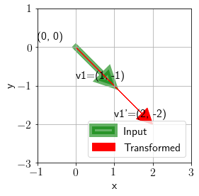
Note that this special vector is not changing direction but only the magnitude. All such special vectors under transformation \(A\) are eigen vectors of \(A\).

We can see that the transformed vector is \(2\) times longer. This denotes that for eigen vector \(\mathbf{e} = [1\;\;\;-1]^T\) corresponding eigen value is \(2\).

Now, let us check for input vector \([1\;\;\;0]^T\),

fig, ax = plt.subplots()
plot_transformation(np.array([1, 0]).reshape(-1,1), np.array([[3, 1], [0, 2]]), ax, annotate=True);

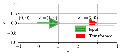
We can see that the transformed vector is \(3\) times longer. This denotes that for eigen vector \(\mathbf{e} = [1\;\;\;0]^T\) corresponding eigen value is \(3\).

Prog-ML

Eigen values

Eigen values¶