Sampling from common distributions

From the ground up!

• toc: true

• badges: true

• comments: true

• author: Nipun Batra

• categories: [ML]

import numpy as np
import matplotlib.pyplot as plt
%matplotlib inline

PRNG

Uniform distribution

I am pasting the code from vega-vis

export default function(seed) {
  // Random numbers using a Linear Congruential Generator with seed value
  // Uses glibc values from https://en.wikipedia.org/wiki/Linear_congruential_generator
  return function() {
    seed = (1103515245 * seed + 12345) % 2147483647;
    return seed / 2147483647;
  };
}

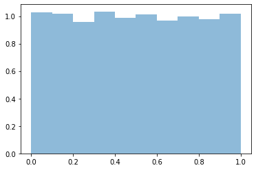
def random_gen(seed, num):
    out = np.zeros(num)
    out[0] =  (1103515245 * seed + 12345) % 2147483647
    for i in range(1, num):
        out[i] = (1103515245 * out[i-1] + 12345) % 2147483647
    return out/2147483647
        
        

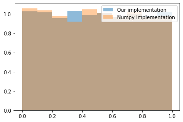
plt.hist(random_gen(0, 5000), density=True, alpha=0.5, label='Our implementation');

plt.hist(random_gen(0, 5000), density=True, alpha=0.5, label='Our implementation');
plt.hist(np.random.random(5000), density=True, alpha=0.4, label='Numpy implementation');
plt.legend()

<matplotlib.legend.Legend at 0x7f51d3cbd290>

Inverse transform sampling

Exponential distribution

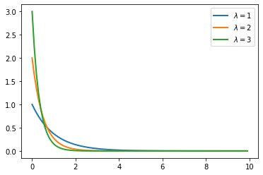
Borrowing from Wikipedia.

The probability density function (pdf) of an exponential distribution is $\( f(x ; \lambda)=\left\{\begin{array}{ll} \lambda e^{-\lambda x} & x \geq 0 \\ 0 & x \leq 0 \end{array}\right. \)$

The exponential distribution is sometimes parametrized in terms of the scale parameter \(\beta=1 / \lambda:\) $\( f(x ; \beta)=\left\{\begin{array}{ll} \frac{1}{\beta} e^{-x / \beta} & x \geq 0 \\ 0 & x<0 \end{array}\right. \)$

The cumulative distribution function is given by $\( F(x ; \lambda)=\left\{\begin{array}{ll} 1-e^{-\lambda x} & x \geq 0 \\ 0 & x<0 \end{array}\right. \)$

from scipy.stats import expon
rvs = [expon(scale=s) for s in [1/1., 1/2., 1/3.]]

x = np.arange(0, 10, 0.1)
for i, lambda_val in enumerate([1, 2, 3]):
    plt.plot(x, rvs[i].pdf(x), lw=2, label=r'$\lambda=%s$' %lambda_val)
plt.legend()

<matplotlib.legend.Legend at 0x7f51da6d4e10>

For the purposes of this notebook, I will be looking only at the standard exponential or set the scale to 1.

Let us now view the CDF of the standard exponential.

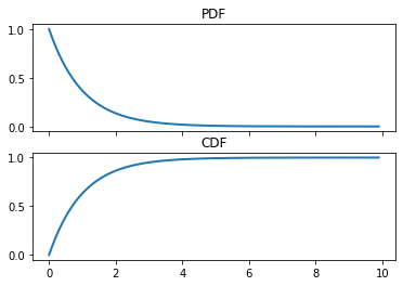
fig, ax = plt.subplots(nrows=2, sharex=True)
ax[0].plot(x, expon().pdf(x), lw=2)
ax[0].set_title("PDF")
ax[1].set_title("CDF")
ax[1].plot(x, expon().cdf(x), lw=2,)

[<matplotlib.lines.Line2D at 0x7f51d8985a90>]

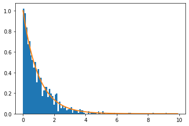
r = expon.rvs(size=1000)

plt.hist(r, normed=True, bins=100)
plt.plot(x, expon().pdf(x), lw=2)

/home/nipunbatra-pc/anaconda3/lib/python3.7/site-packages/ipykernel_launcher.py:1: MatplotlibDeprecationWarning: 
The 'normed' kwarg was deprecated in Matplotlib 2.1 and will be removed in 3.1. Use 'density' instead.
  """Entry point for launching an IPython kernel.

[<matplotlib.lines.Line2D at 0x7f51d86b5ad0>]

Inverse of the CDF of exponential

The cumulative distribution function is given by $\( F(x ; \lambda)=\left\{\begin{array}{ll} 1-e^{-\lambda x} & x \geq 0 \\ 0 & x<0 \end{array}\right. \)$

Let us consider only \(x \geq 0\).

Let \(u = F^{-1}\) be the inverse of the CDF of \(F\).

\[\begin{split} u = 1-e^{-\lambda x} \\ 1- u = e^{-\lambda x} \\ \log(1-u) = -\lambda x\\ x = -\frac{\log(1-u)}{\lambda} \end{split}\]

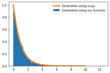
def inverse_transform(lambda_val, num_samples):
    u = np.random.random(num_samples)
    x = -np.log(1-u)/lambda_val
    return x

plt.hist(inverse_transform(1, 5000), bins=100, normed=True,label='Generated using our function');
plt.plot(x, expon().pdf(x), lw=4, label='Generated using scipy')
plt.legend()

/home/nipunbatra-pc/anaconda3/lib/python3.7/site-packages/ipykernel_launcher.py:1: MatplotlibDeprecationWarning: 
The 'normed' kwarg was deprecated in Matplotlib 2.1 and will be removed in 3.1. Use 'density' instead.
  """Entry point for launching an IPython kernel.

<matplotlib.legend.Legend at 0x7f51d5f95410>

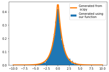
Drawing samples from Laplace distribution

A random variable has a Laplace \((\mu, b)\) distribution if its probability density function is $\( f(x | \mu, b)=\frac{1}{2 b} \exp \left(-\frac{|x-\mu|}{b}\right) \)$

\[F^{-1}(u)=\mu-b \operatorname{sgn}(u-0.5) \ln (1-2|u-0.5|)\]

def inverse_transform_laplace(b, mu, num_samples):
    u = np.random.random(num_samples)
    x = mu-b*np.sign(u-0.5)*np.log(1-2*np.abs(u-0.5))
    return x

from scipy.stats import laplace
plt.hist(inverse_transform_laplace(1, 0, 5000),bins=100, density=True, label='Generated using \nour function');
x_n = np.linspace(-10, 10, 100)
plt.plot(x_n, laplace().pdf(x_n), lw=4, label='Generated from\n scipy')
plt.legend()

<matplotlib.legend.Legend at 0x7f51d4a99750>

Box-Muller transform