Bayesian ML: Fundamentals

Author: Zeel B Patel

import numpy as np
import pandas as pd
import matplotlib.pyplot as plt
from matplotlib import rc
from matplotlib.animation import FuncAnimation
from mpl_toolkits import mplot3d
from jax import numpy as jnp, grad
import scipy

What is the intuition behind the Bayesian update?

https://www.youtube.com/watch?v=HZGCoVF3YvM

Guess who is Steve? A farmer or a librarian?

Paradox in the above example suggests noting the essense of Bayes rule as the following,

• New information does not completely determine the new belief but it just updates the prior belief

Bayes theorem

\[ p(B|A) = \frac{p(A|B)}{p(A)}p(B) \to p(\theta|D) = \frac{p(D|\theta)}{p(D)}p(\theta) \]

• \(p(D|\theta)\) - likelihood

• \(p(\theta)\) - prior

• \(p(D)\) - evidence

• \(p(\theta|D)\) - posterior

Let us understand Likelihood, prior and evidence individually then we will move to the posterior

Likelihood and Maximum Likelihood estimation (MLE)

import numpy as np
import matplotlib.pyplot as plt
from matplotlib import rc
from matplotlib.animation import FuncAnimation

rc('font',size=16)
rc('text',usetex=True)

What is the likelihood? How likely the event is, given a belief. It is defined as below in the ML context.

\[ p(D|\theta) \]

A simple coin flip experiment.

We want to determine the probability (likelihood) of \(D=\{H,T,H,H,H,H,T,H,H,H\}\) after 10 coin flips believing that we have a fair coin (\(p(H)=\theta=0.5\)).

\[ p(D|\theta) = \prod\limits_{i=1}^{10}p(D_i|\theta) = (0.5)^8(0.5)^2 = 2^{-10} \]

More generally, out of N experiments, if we see \(h\) heads, likelihood \(p(D|\theta)\) is,

\[ p(D|\theta) = (\theta)^h(1-\theta)^{N-h} \]

This likelihood is known as the Bernoulli likelihood.

In the aboce example, \(D\) event is less likely given a fair coin. Intuitively, looking at \(D\), the coin seems biased towards \(H\)? What’s your guess for \(\theta\)?

Let’s visualize likelihood of \(D\) for various values of \(\theta\).

def Bernoulli(theta,N,h):
    return (theta**h)*((1-theta)**(N-h))
def BernoulliModified(theta,N,h): # exp after log
    return np.exp(h*np.log(theta) + (N-h)*np.log(1-theta))
def LogBernoulli(theta,N,h): # exp after log
    return h*np.log(theta) + (N-h)*np.log(1-theta)

N,h = 10,8
theta = np.linspace(0.01,0.99,100)
BL = [Bernoulli(t,N,h) for t in theta]
BLM = BernoulliModified(theta,N,h)
LogBL = LogBernoulli(theta,N,h)
fig, ax = plt.subplots(figsize=(10,4))
ax.plot(theta, BL);
plt.xlabel('$\\theta$');plt.ylabel('Likelihood $p(D|\\theta)$');
plt.title('Likelihood of observing $D=\{H,T,H,H,H,H,T,H,H,H\}$');

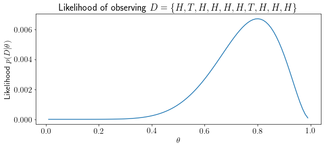
Visually, we can see that, our event is most likely at \(\theta=0.8\). How can we say that concretely (with mathematical/analytical support)?

We need to look at the maximum likelihood for this problem.

Maximum likelihood estimation (MLE)

We know that following claims are true for any differentiable function,

• \(\theta\) would be optimal at \(\frac{d}{d\theta}L(D|\theta)=0\)

• \(\theta\) would be maximum at \(\frac{d^2}{d\theta^2}L(D|\theta)<0\).

Let us find out optimal \(\theta\) using the above propoerties.

(1)\[\begin{align} p(D|\theta) &= (\theta)^h(1-\theta)^{N-h}\\ \frac{d}{d\theta}p(D|\theta) &= h\theta^{h-1}(1-\theta)^{N-h} - (N-h)\theta^h(1-\theta)^{N-h-1} = 0\\ \\ \text{follows that,}\\ h(1-\theta)-(N-h)\theta &= 0\\ h - h\theta - N\theta + h\theta &= 0\\ \theta_{MLE} &= \frac{h}{N} \end{align}\]

Verifying our example, we had \(h=8\) and \(N=10\), so \(\theta_{MLE}=8/10=0.8\).

We see from the earlier plot that this is a maxima, but one can also verify it by double differentiation.

Likelihood v/s modified likelihood v/s log likelihood

Bernoulli likelihood is given as following,

\[ p(D|\theta) = (\theta)^h(1-\theta)^{N-h} \]

We can avoid potential numerical errors transforming it as following,

\[ p(D|\theta) = \exp\left[h\log(\theta)+(N-h)\log(1-\theta)\right] \]

Or, we can use the log-likelihood directly.

\[ \log p(D|\theta) = h\log(\theta)+(N-h)\log(1-\theta) \]

Let us visualize these three variants for our coin toss example.

def Bernoulli(theta,N,h):
    return (theta**h)*((1-theta)**(N-h))
def BernoulliModified(theta,N,h): # exp after log
    return np.exp(h*np.log(theta) + (N-h)*np.log(1-theta))
def LogBernoulli(theta,N,h): # exp after log
    return h*np.log(theta) + (N-h)*np.log(1-theta)

N,h = 10,8
theta = np.linspace(0.01,0.99,100)
BL = [Bernoulli(t,N,h) for t in theta]
BLM = BernoulliModified(theta,N,h)
LogBL = LogBernoulli(theta,N,h)

fig, ax = plt.subplots(1,3,figsize=(15,4))
ax[0].plot(theta, BL);
ax[1].plot(theta, BLM);
ax[2].plot(theta, LogBL);
for axs in ax:
    axs.set_xlabel('$\\theta$')
    axs.vlines(0.8,*axs.get_ylim(),linestyle='--', label='MLE')
ax[0].text(0,0.0005,'Almost zero')
ax[1].text(0,0.0005,'Almost zero')
ax[0].legend()
ax[0].set_title('Likelihood');
ax[1].set_title('Modified likelihood');
ax[2].set_title('Log likelihood');

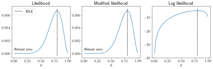
What are the benefits of using log likelihood over likelihood?

• Avoids numerical underflow/overflow

• Handles close to zero values efficiently.

MLE with log likelihood

Stating the optimization rules for log likelihood

• \(\theta\) would be optimal at \(\frac{d}{d\theta}\log L(D|\theta)=0\)

• \(\theta\) would be maximum at \(\frac{d^2}{d\theta^2}\log L(D|\theta)<0\).

(2)\[\begin{align} p(D|\theta) &= (\theta)^h(1-\theta)^{N-h}\\ \log p(D|\theta) &= h\log(\theta)+(N-h)\log(1-\theta)\\ \frac{d}{d\theta}\log p(D|\theta) &= \frac{h}{\theta} - \frac{N-h}{1-\theta} = 0\\ \\ \text{follows that,}\\ h(1-\theta)-(N-h)\theta &= 0\\ h - h\theta - N\theta + h\theta &= 0\\ \theta_{MLE} &= \frac{h}{N} \end{align}\]

Notice that double differentiation is trivial in this setting,

(3)\[\begin{align} \frac{d}{d\theta}\log p(D|\theta) &= \frac{h}{\theta} - \frac{N-h}{1-\theta}\\ \frac{d^2}{d\theta^2}\log p(D|\theta) &= -\frac{h}{\theta^2}-\frac{N-h}{(1-\theta)^2} < 0 \end{align}\]

Double differentiation is negative and thus our optima is the maxima.

Now onwards, we will directly use log likelihood.

Gaussian distribution

A continuous random variable is called Gaussian distributed if it follows the below pdf,

\[ p(x|\mu,\sigma) = \frac{1}{\sqrt{2\pi\sigma^2}}exp\left[{-\frac{(x-\mu)^2}{2\sigma^2}}\right] \]

Let’s visualize some samples drawn from Gaussian distribution.

rc('font',size=20)
rc('text',usetex=True)
np.random.seed(0)
x = np.random.normal(10,2,size=100)
plt.figure(figsize=(15,4))
plt.eventplot(x);
plt.yticks([]);plt.xlabel('x');
plt.title('What should be $\mu$? What should be $\sigma$?');

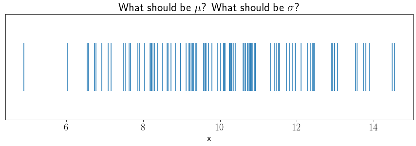
Hold this question for now, first, let us visualize the pdf of Gaussian distribution by varying \(\mu\) and \(\sigma\).

def GaussianPDF(mu, sigma, x):
    return (1/np.sqrt(2*np.pi*sigma**2))*np.exp(-np.square(x-mu)/2/sigma**2)

rc('font',size=16)
rc('text',usetex=True)
fig, ax = plt.subplots(figsize=(10,4))
mu, sigma = 0, 10
def update(mu):
    np.random.seed(mu)
    ax.cla()
    x = np.sort(np.random.normal(mu, sigma, 100))
    pdfx = np.linspace(x.min(), x.max(), 100)
    G_pdf = GaussianPDF(mu, sigma, pdfx)
    ax.plot(pdfx, G_pdf,label='pdf')
    ax.plot(x, np.ones(x.shape[0])*-0.001, '|k', markersize=20, label='samples')
    ax.vlines([mu+sigma, mu-sigma], *ax.get_ylim(), label='$\sigma$', linestyle='--')
    ax.vlines([mu+2*sigma, mu-2*sigma], *ax.get_ylim(), label='$2\sigma$', linestyle='--',color='r')
    ax.legend()
    ax.set_xlabel('x');ax.set_ylabel('pdf');
    ax.set_title(f'$\mu$ = {mu}, $\sigma$={sigma}');
    ax.set_xlim(-35,90)
    plt.tight_layout()
plt.close()
anim = FuncAnimation(fig, update, frames=np.arange(1,60,5))
rc('animation',html='jshtml')
anim

Once Loop Reflect

<Figure size 432x288 with 0 Axes>

def GaussianPDF(mu, sigma, x):
    return (1/np.sqrt(2*np.pi*sigma**2))*np.exp(-np.square(x-mu)/2/sigma**2)

rc('font',size=16)
rc('text',usetex=True)
fig, ax = plt.subplots(figsize=(10,4));
mu, sigma = 0, 10
def update(sigma):
    np.random.seed(0)
    ax.cla()
    x = np.sort(np.random.normal(mu, sigma, 100))
    pdfx = np.linspace(x.min(), x.max(), 100)
    G_pdf = GaussianPDF(mu, sigma, pdfx)
    ax.plot(pdfx, G_pdf,label='pdf')
    ax.plot(x, np.ones(x.shape[0])*-0.001, '|k', markersize=20, label='samples')
    ax.vlines([mu+sigma, mu-sigma], *ax.get_ylim(), label='$\sigma$', linestyle='--')
    ax.vlines([mu+2*sigma, mu-2*sigma], *ax.get_ylim(), label='$2\sigma$', linestyle='--',color='r')
    ax.legend()
    ax.set_xlabel('x');ax.set_ylabel('pdf');
    ax.set_title(f'$\mu$ = {mu}, $\sigma$={sigma}');
    ax.set_xlim(-35,35)
    ax.set_ylim(-0.02,0.12)
    plt.tight_layout();

plt.close();
anim = FuncAnimation(fig, update, frames=np.arange(4,11))
anim

Once Loop Reflect

<Figure size 432x288 with 0 Axes>

MLE estimate for the Gaussian distribution parameters

We draw N samples independently from a Gaussian distribution. \(D=\{x_1, x_2, ..., x_N\}\)

Let us estimate \(\mu_{MLE}\) first,

(4)\[\begin{align} p(D|\mu) &= \prod\limits_{i=1}^{N}\frac{1}{\sqrt{2\pi\sigma^2}}exp\left[{-\frac{(x_i-\mu)^2}{2\sigma^2}}\right]\\ \log p(D|\mu) &= -\frac{N}{2}\log(2\pi\sigma^2)-\frac{1}{2}\sum\limits_{i=1}^{N}\frac{(x_i-\mu)^2}{\sigma^2}\\ \frac{d}{d\mu}\log p(D|\mu) &= \sum\limits_{i=1}^{N}\frac{(x_i-\mu)}{\sigma^2} = 0\\ \\ \text{Follows that,}\\ \mu_{MLE} &= \frac{1}{N}\sum\limits_{i=1}^{N}x_i \end{align}\]

Now, we will estimate \(\sigma_{MLE}\),

(5)\[\begin{align} p(D|\sigma) &= \prod\limits_{i=1}^{N}\frac{1}{\sqrt{2\pi\sigma^2}}exp\left[{-\frac{(x_i-\mu)^2}{2\sigma^2}}\right]\\ \log p(D|\sigma) &= -\frac{N}{2}\log(2\pi\sigma^2)-\frac{1}{2}\sum\limits_{i=1}^{N}\frac{(x_i-\mu)^2}{\sigma^2}\\ \frac{d}{d\sigma}\log p(D|\sigma) &= -\frac{N}{2}\frac{4\pi\sigma}{2\pi\sigma^2} + \sum\limits_{i=1}^{N}\frac{(x_i-\mu)^2}{\sigma^3} = 0\\ \\ \text{Follows that,}\\ \frac{N}{\sigma} &= \sum\limits_{i=1}^{N}\frac{(x_i-\mu)^2}{\sigma^3}\\ \sigma^2_{MLE} &= \frac{1}{N}\sum\limits_{i=1}^{N}(x_i-\mu)^2 \end{align}\]

Let us estimate MLE of \(\mu, \sigma\) for the samples shown earlier.

def LogGaussian(mu, sigma, x):
    return -0.5*np.log(2*np.pi*sigma**2)*x.shape[0] - 0.5*np.sum(np.square((x.squeeze()-mu)/sigma))

mu,sigma=10,3
np.random.seed(0)
x = np.random.normal(10,2,size=100)
muR = np.linspace(1,18,100)
Lmu = [LogGaussian(mu, sigma, x) for mu in muR]
Lsigma = [LogGaussian(mu, sigma, x) for sigma in muR]

rc('font',size=18)
rc('text',usetex=True)
fig, ax = plt.subplots(3,1,figsize=(12,8), sharex=True)
ax[0].plot(muR, Lmu);ax[0].set_ylabel('log likelihood\nover $\mu$');
ax[1].plot(muR, Lsigma, color='r')
ax[1].set_ylabel('log likelihood\nover $\sigma$');
ax[0].set_title('Log likelihood');ax[0].set_xlabel('$\mu$');ax[1].set_xlabel('$\sigma$');
ax[0].vlines(np.mean(x), *ax[0].get_ylim(), linestyle='--',label='$\mu_{MLE}$')
ax[1].vlines(np.std(x), *ax[0].get_ylim(), linestyle='--',label='$\sigma_{MLE}$',color='r')
ax[2].eventplot(x);ax[2].set_xlabel('x');ax[2].set_ylabel('Number of points');
ax[2].vlines(np.mean(x), *ax[2].get_ylim(), linestyle='--',label='$\mu_{MLE}$')
ax[2].vlines([np.mean(x)-np.std(x),np.mean(x)+np.std(x)], *ax[2].get_ylim(), linestyle='--',label='$\mu_{MLE}\pm\sigma_{MLE}$',color='r')
ax[2].set_title('Samples');
for axs in ax:
    axs.legend(bbox_to_anchor=(1.3,1));
plt.tight_layout();

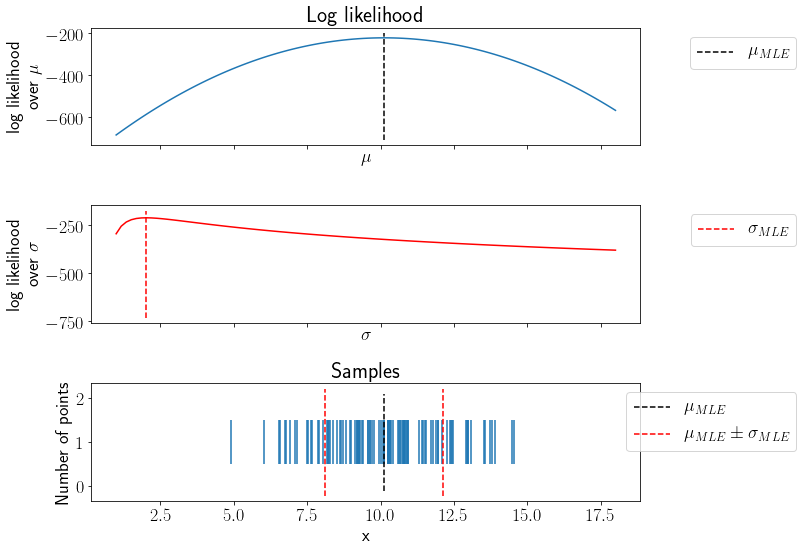
Notice the mean and standard deviation values in above plot. Let us verify this result analytically,

np.mean(x), np.std(x)

(10.11961603106897, 2.0157644894331592)

Poisson distribution

A discrete random variable is called Poisson distributed if it has the following pmf,

\[ p(x|\lambda) = \frac{\lambda^xe^{-\lambda}}{x!} \]

Wonder how this formula is derived? checkout https://www.youtube.com/watch?v=7cg-rxofqj8

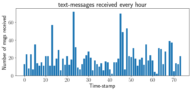
A potential application can be modeling text-messages given in this book.

msg = np.loadtxt('https://raw.githubusercontent.com/CamDavidsonPilon/Probabilistic-Programming-and-Bayesian-Methods-for-Hackers/master/Chapter1_Introduction/data/txtdata.csv')
plt.figure(figsize=(10,4))
plt.bar(range(len(msg)),msg);
plt.title('text-messages received every hour');
plt.xlabel('Time-stamp');plt.ylabel('Number of msgs received');

Other applications

1. Telephone calls arriving in a system

2. Customers arriving at a counter

3. The number of photons emitted in a single laser pulse

And many more on Wikipedia

The following animation shows how pmf varies with varying \(\lambda\).

def Poisson(lmd, k):
    return lmd**k*np.exp(-lmd)/np.math.factorial(int(k))

k = np.arange(21)
rc('font',size=14)
fig, axs = plt.subplots(1,2,figsize=(12,5))
ax, ax1 = axs
def update(lmd):
    np.random.seed(0)
    ax.cla();ax1.cla()
    P_pdf = [Poisson(lmd, ki) for ki in k]
    ax.plot(k, P_pdf,'o-',label='pmf')
    ax.set_xlabel('x');ax.set_ylabel('pmf');
    ax.set_title(f'lambda = {lmd}')
    ax.set_ylim(0,0.4);
    ax.legend();
    
    ax1.bar(range(20), np.random.poisson(lam=lmd, size=20))
    ax1.set_title('Samples')
    ax1.set_ylim(0,20);
plt.close()
anim = FuncAnimation(fig, update, frames=np.arange(1,11))
rc('animation',html='jshtml')
anim

Once Loop Reflect

MLE estimate for the Poisson distribution parameters

We draw N samples independently from a Poisson distribution. \(D=\{x_1, x_2, ..., x_N\}\),

(6)\[\begin{align} p(D|\lambda) &= \prod\limits_{i=1}^{N}\frac{\lambda^{x_i}e^{-\lambda}}{x_i!}\\ \log p(D|\lambda) &= \sum\limits_{i=1}^{N}\log(\lambda^{x_i})+\sum\limits_{i=1}^{N}\log(e^{- \lambda})-\sum\limits_{i=1}^{N}\log(x_i!)\\ \frac{d}{d\lambda}\log p(D|\lambda) &= \frac{\sum\limits_{i=1}^{N}x_i}{\lambda} - \sum\limits_{i=1}^{N}1 = 0\\ \lambda_{MLE} &= \frac{1}{N}\sum\limits_{i=1}^{N}x_i \end{align}\]

Let us estimate MLE of \(\lambda\) for the text-messages data.

np.random.seed(123)
x = msg
L = [np.sum([np.log(Poisson(lmdi, xi)) for xi in x]) for lmdi in range(1,60)]
rc('font',size=20)
fig, ax = plt.subplots(1,2,figsize=(12,4))
ax[0].plot(range(1,60), L);ax[0].set_xlabel('$\lambda$');ax[0].set_ylabel('log likelihood');
ax[0].set_title('Log likelihood $p(D|\lambda)$');
ax[0].vlines(np.mean(x), *ax[0].get_ylim(), linestyle='--',label='MLE')
ax[1].bar(range(len(msg)), msg);ax[1].set_xlabel('Time-stamps');ax[1].set_ylabel('Number of points');
ax[1].set_title('Number of msg per hour');
ax[0].legend(bbox_to_anchor=(1,0.3));

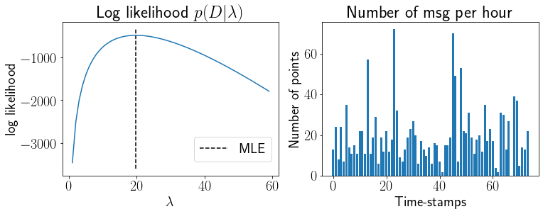
np.mean(x)

19.743243243243242

You should trust MLE with a caution..!!

Bayes Rule: New evidence does not completely determine the new belief but it updates the prior belief.

According to MLE,

• \(D=\{H,H,H,H\} \to \theta_{MLE}=1\)

• \(D=\{H,T,T,H\} \to \theta_{MLE}=0.5\)

• \(D=\{T,T,T,T\} \to \theta_{MLE}=0\)

Thus, we need to consider a prior belief in our parameter estimation

Prior beliefs over parameters

Before moving to prior over parameters, we will see what is a Beta distribution (we will use it later in the flow).

Beta distribution

pdf of Beta distribution is defined as,

\[\begin{split} p(\theta|\alpha, \beta) = \frac{\theta^{\alpha-1}(1-\theta)^{\beta-1}}{B(\alpha,\beta)}, \alpha,\beta>0\\ B(\alpha, \beta) = \frac{\Gamma(\alpha)\Gamma(\beta)}{\Gamma(\alpha+\beta)}\\ \Gamma(\alpha) = (\alpha-1)! \end{split}\]

The following animation shows effect of varying \(\alpha, \beta\) on the pdf.

theta = np.linspace(0,1,50)
alp = np.linspace(1,5,10).tolist() + np.linspace(5,5,10).tolist() + np.linspace(5,1,10).tolist() + np.linspace(1,10,10).tolist() + np.linspace(10,1,10).tolist() + np.linspace(1,0.1,10).tolist()
bet = np.linspace(5,5,10).tolist() + np.linspace(5,1,10).tolist() + np.linspace(1,1,10).tolist() + np.linspace(1,10,10).tolist() + np.linspace(10,1,10).tolist() + np.linspace(1,0.1,10).tolist()

fig, ax = plt.subplots(figsize=(6,5));
def update(i):
    ax.cla();
    ax.plot(theta, scipy.stats.beta.pdf(theta, alp[i], bet[i]));
    ax.set_title(f'$\\alpha$={np.round(alp[i],2)}, $\\beta$ = {np.round(bet[i],2)}');
    ax.set_ylim(0,6);
    ax.set_xlabel('$\\theta$');ax.set_ylabel('pdf');
    plt.tight_layout();

plt.close();
anim = FuncAnimation(fig, update, range(len(alp)));
anim

Once Loop Reflect

<Figure size 432x288 with 0 Axes>

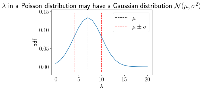
Parameters may have an underlying distribution

x = np.linspace(0,20,21)
Gaussprior = GaussianPDF(7, 3, x)
rc('font',size=20)
plt.plot(x, Gaussprior);
plt.vlines(7,*plt.gca().get_ylim(), linestyle='--', label='$\mu$')
plt.vlines([7-3,7+3],*plt.gca().get_ylim(), linestyle='--', label='$\mu\pm\sigma$',color='r')
plt.title('$\lambda$ in a Poisson distribution may have a Gaussian distribution $\mathcal{N}(\mu,\sigma^2)$');
plt.xlabel('$\lambda$');plt.ylabel('pdf');
plt.legend();

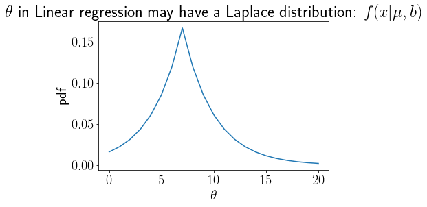
def LaplacePDF(mu, b, x):
    return (1/2/b)*np.exp(-np.abs(x - mu)/b)

x = np.linspace(0,20,21)
Laplaceprior = LaplacePDF(7, 3, x)
rc('font',size=20)
plt.plot(x, Laplaceprior);
plt.title('$\\theta$ in Linear regression may have a Laplace distribution: $f(x|\mu,b)$');
plt.xlabel('$\\theta$');plt.ylabel('pdf');

How to choose appropriate prior distribution for given likelihood ? \(\to\) Conjugate priors

We choose a conjugate prior to likelihood to ensure the same distribution in posterior as prior

• Example 1: Bernoulli likelihood \(\to\) Beta prior \(\to\) Beta posterior

• Example 2: Gaussian likelihood \(\to\) Gaussian prior \(\to\) Gaussian posterior

More info on conjugate priors is at https://en.wikipedia.org/wiki/Conjugate_prior

Maximum A Posteriori (MAP) estimation

Utilizing prior distribution, we can get more realistic (in Bayesian sense) estimate of parameters compared to MLE. We will call this MAP.

(7)\[\begin{align} p(\theta_{posterior}|D) &= \frac{p(D|\theta_{prior})}{p(D)}p(\theta_{prior})\\ p(D) \text{ can be treated as a constant}\\ p(\theta_{posterior}|D) &\propto p(D|\theta_{prior})p(\theta_{prior}) \\\\ \text{MLE: }&\arg\max_\theta \; p(D|\theta)\\ \text{MAP: }&\arg\max_\theta \; p(\theta|D) = \arg\max_\theta \; p(D|\theta)p(\theta) \end{align}\]

MAP for a simple coin flip experiment

We assume \(p(\theta) \sim Beta(\alpha, \beta)\) (Because Beta prior is conjugate to Bernoulli likelihood)

(8)\[\begin{align} p(\theta|D)p(\theta) &= \theta^h(1-\theta)^{N-h}\cdot\frac{\theta^{\alpha-1}(1-\theta)^{\beta-1}}{B(\alpha, \beta)}\\ &= \frac{\theta^{h+\alpha-1}(1-\theta)^{N-h+\beta-1}}{B(\alpha, \beta)}\\ \log p(\theta|D)p(\theta) &= (h+\alpha-1)\log(\theta) + (N-h+\beta-1)\log(1-\theta) - \log(B(\alpha, \beta))\\ \\ \frac{d}{d\theta} \log p(\theta|D)p(\theta) &= \frac{h+\alpha-1}{\theta} - \frac{N-h+\beta-1}{1-\theta} = 0\\ \\ \theta_{MAP} &= \frac{h+(\alpha-1)}{N+(\alpha-1)+(\beta-1)} \end{align}\]

Let us visualize MLE and MAP for various prior (effectively varying \(\alpha,\beta\) of Beta prior)

N,h = 10,8
theta = np.linspace(0.01,0.99,100)
BL = [Bernoulli(t,N,h) for t in theta]
BLM = BernoulliModified(theta,N,h)
LogBL = LogBernoulli(theta,N,h)
rc('font',size=20)
rc('text',usetex=True)
fig, ax = plt.subplots(figsize=(10,4))
axs = ax.twinx()
def update(i):
    ax.cla();axs.cla();
    axs.set_ylim(-0.02,5)
    al,be = alp[i], bet[i]
    ax.plot(theta, BL, label='Likelihood',color='b');
    axs.plot(theta, scipy.stats.beta.pdf(theta, al,be), label='Prior',color='k');
    ax.set_xlabel('$\\theta$');
    ax.vlines(0.8, *ax.get_ylim(), linestyle='--',label='MLE',color='b')
    ax.text(0.8,0,'MLE',color='b')
    ax.text(theta[0], BL[0],'Likelihood',color='b')
    axs.text(theta[0], scipy.stats.beta.pdf(theta, al,be)[0],'Prior',color='k')
    axs.text(al/(al+be)-0.1,2,'Prior mean',color='k')
    axs.text((h+al-1)/(N+al+be-2),1,'MAP',color='r')
    ax.vlines(al/(al+be), *ax.get_ylim(), linestyle='--',label='Prior mean',color='k')
    ax.vlines((h+al-1)/(N+al+be-2), *ax.get_ylim(), linestyle='--',label='MAP',color='r')
    ax.set_title('D=\{H,T,H,H,H,H,T,H,H,H\}, $\\alpha = '+str(np.round(al,2))+'$, $\\beta='+str(np.round(be,2))+'$');
    # ax.set_yscale('log');
#     ax.legend(bbox_to_anchor=(1,1));axs.legend(bbox_to_anchor=(1.25,0.6));
plt.tight_layout()
plt.close()
anim = FuncAnimation(fig, update, range(len(alp)))
anim

Once Loop Reflect

Evidence \(p(D)\)

Note that we discussed about likelihood and prior. If we get the evidence (denominator in Bayes formula) as well, we can compute the exact posterior distribution.

\[ p(D) = \int\limits_{\theta}p(D|\theta)p(\theta)d\theta \]

\[ p(D) = \sum\limits_{\theta\in \Theta}p(D|\theta)\theta \]

In practive, evidence is hard to calculate because of non-trivial intigration over \(\theta\). But, in simple models, it is possible to derive.

Full posterior calculation for coin toss experiment

(9)\[\begin{align} p(D) &= \int\limits_{0}^{1}p(D|\theta)p(\theta)d\theta\\ &= \int\limits_{0}^{1}(\theta)^h(1-\theta)^{N-h}\frac{\theta^{\alpha-1}(1-\theta)^{\beta-1}}{B(\alpha,\beta)}d\theta\\ &= \frac{1}{B(\alpha,\beta)}\int\limits_{0}^{1}(\theta)^{h+\alpha-1}(1-\theta)^{N-h+\beta-1}\\ &= \frac{1}{B(\alpha,\beta)}\frac{(h+\alpha-1)!(N-h+\beta-1)!}{(N+\alpha+\beta-1)!} \end{align}\]

(10)\[\begin{align} p(\theta|D) = \frac{p(D|\theta)}{p(D)}p(\theta)&=B(\alpha,\beta)\frac{(N+\alpha+\beta-1)!}{(h+\alpha-1)!(N-h+\beta-1)!}\frac{\theta^{h+\alpha-1}(1-\theta)^{N-h+\beta-1}}{B(\alpha, \beta)}\\ \\ &= Beta(h+\alpha, N-h+\beta) \end{align}\]

We have successfully shown that the posterior follows Beta distribution. Let us visualize the exact posterior distribution.

from scipy.special import gamma

N,h = 10,8
theta = np.linspace(0.01,0.99,100)
BL = [Bernoulli(t,N,h) for t in theta]
BLM = BernoulliModified(theta,N,h)
LogBL = LogBernoulli(theta,N,h)
rc('font',size=20)
rc('text',usetex=True)
fig, ax = plt.subplots(figsize=(10,4))
axs = ax.twinx()
def update(i):
    ax.cla();axs.cla()
    axs.set_ylim(-0.02,5)
    al,be = alp[i], bet[i]
    ax.plot(theta, BL, label='Likelihood',color='b');
    axs.plot(theta, scipy.stats.beta.pdf(theta, al,be), label='Prior',color='k');
    ax.set_xlabel('$\\theta$');
    ax.vlines(0.8, *ax.get_ylim(), linestyle='--',label='MLE', color='b')
    axs.text(0.8,2,'MLE', color='b')
    
    axs.plot(theta, [scipy.stats.beta.pdf(t, h+al, N-h+be) for t in theta], color='r')
    ax.text(theta[0], BL[0],'Likelihood', color='b')
    axs.text(theta[0], scipy.stats.beta.pdf(theta, al,be)[0],'Prior')
    axs.text(al/(al+be)-0.1,2,'Prior mean')
    axs.text(theta[0],scipy.stats.beta.pdf(theta[0], h+al, N-h+be),'Posterior',color='r')
    axs.text((h+al)/(N+al+be)-0.1,1,'Post. Mean',color='r')
    ax.vlines(al/(al+be), *ax.get_ylim(), linestyle='--',label='Prior mean',color='k')
#     ax.vlines((h+al-1)/(N+al+be-2), *ax.get_ylim(), linestyle='--',label='MAP',color='r')
    ax.vlines((h+al)/(N+al+be), *ax.get_ylim(), linestyle='--',label='Post. Mean',color='r')
    ax.set_title('D=\{H,T,H,H,H,H,T,H,H,H\}, $\\alpha = '+str(np.round(al,2))+'$, $\\beta='+str(np.round(be,2))+'$');
    # ax.set_yscale('log');
#     ax.legend(bbox_to_anchor=(1,1));axs.legend(bbox_to_anchor=(1.25,0.6));
plt.tight_layout()
plt.close()
anim = FuncAnimation(fig, update, range(len(alp)))
anim

Once Loop Reflect

Another use of evidence \(p(D)\) is model comparison. For multiple models, higher value of \(p(D)\) suggests a better model.

\[ BayesFactor = \frac{p(D|M1)}{p(D|M2)} \]

We will look into this aspect in other notebooks.

MAP is not always mean of the posterior

We have derived the MAP for our problem as:

\[ \theta_{MAP} = \frac{h+(\alpha-1)}{N+(\alpha-1)+(\beta-1)} \]

However, mean of our posterior distribution is: $\( \theta_{Post. Mean} = \frac{h+\alpha}{N+\alpha+\beta} \)$

Why do we care? Because MAP matters when we are just interested in maximum probable value of \(\theta\) from the posterior and the distribution matters when we want to use it for further computation or analyse its properties such a mean and variance.