
Sample Space and Random Variables
Contents
Sample Space and Random Variables#
Inspired by: MIT Open Course
Common packages#
import jax  # numpy on steroids: autograd, GPU/TPU acceleration and other tricks
import jax.numpy as jnp  # jax's own numpy
import distrax  # distributions in jax
What is a Sample Space?#
A set of all possible outcomes of an experiment. Notation: \(\Omega\)
Mutually exclusive - only one outcome should be possible at the end of an experiment
Collectively exhaustive - togather, elements of sample space exhaust all the possible outcomes of an experiment
Right granularity - Example: Coin toss in a rainy season.
Programmatically constructing sample space#
Draw sufficiently many samples from an experiment (exhaustive)
Consider only unique outcomes (a set of all outcomes)
Example 1: Coin toss#
\(\Omega = \{H, T\}\)
Head (\(H\)) \(\to 1\)
Tail (\(T\)) \(\to 0\)
\(\Omega = \{1, 0\}\)
# Instantiate a Bernolli distribution
coin = distrax.Bernoulli(probs=0.8)  # probability of "Head" is 0.8
WARNING:absl:No GPU/TPU found, falling back to CPU. (Set TF_CPP_MIN_LOG_LEVEL=0 and rerun for more info.)
key = jax.random.PRNGKey(0)
n_samples = 20

# Sample from the distribution
samples = coin.sample(seed=key, sample_shape=n_samples)
print(f"Samples:\n{samples}")
Samples:
[0 1 1 1 0 1 1 1 1 0 1 0 1 1 1 0 1 1 0 1]
sample_space = jnp.unique(samples)
print(f"Sample Space: {sample_space}")
Sample Space: [0 1]
Example 2: Tossing two coins#
two_coins = distrax.Bernoulli(probs=(0.5, 0.6))
key = jax.random.PRNGKey(0)
n_samples = 10

# Sample from the distribution
samples = two_coins.sample(seed=key, sample_shape=n_samples)
print(f"Samples:\n{samples}")
Samples:
[[0 1]
 [1 1]
 [0 1]
 [1 1]
 [0 0]
 [1 0]
 [1 1]
 [0 0]
 [1 0]
 [0 1]]
sample_space = jnp.unique(samples, axis=0)
print(f"Sample Space:\n{sample_space}")
Sample Space:
[[0 0]
 [0 1]
 [1 0]
 [1 1]]
What is an Event?#
An event is a subset of the sample space
Experiment: Tossing two coins
Event: “At least one Head”: \(\{(0, 1), (1, 0), (1, 1)\}\)
Example 3: Roll a die#
die = distrax.Categorical(probs=[1/6]*6)
die.num_categories
6
key = jax.random.PRNGKey(0)
n_samples = 20

# Sample from the distribution
samples = die.sample(seed=key, sample_shape=n_samples)
print(f"Samples:\n{samples}")
Samples:
[2 1 1 3 4 2 4 2 5 5 0 0 4 5 1 1 4 1 0 5]
sample_space = set(samples.tolist())
print(f"Sample Space: {sample_space}")
Sample Space: {0, 1, 2, 3, 4, 5}
Q: What could be an example event in a die roll?
A: “all outcomes with even numbers”
Example 4: Roll two dice#
dice = distrax.Categorical(probs=[[1/4]*6, [1/4]*6])
dice.num_categories
6
dice.batch_shape
(2,)
key = jax.random.PRNGKey(1)
n_samples = 3000

# Sample from the distribution
samples = dice.sample(seed=key, sample_shape=n_samples)
sample_space = jnp.unique(samples, axis=0)
print(f"Sample Space: {sample_space.tolist()}")
Sample Space: [[0, 0], [0, 1], [0, 2], [0, 3], [0, 4], [0, 5], [1, 0], [1, 1], [1, 2], [1, 3], [1, 4], [1, 5], [2, 0], [2, 1], [2, 2], [2, 3], [2, 4], [2, 5], [3, 0], [3, 1], [3, 2], [3, 3], [3, 4], [3, 5], [4, 0], [4, 1], [4, 2], [4, 3], [4, 4], [4, 5], [5, 0], [5, 1], [5, 2], [5, 3], [5, 4], [5, 5]]
Discrete Sample Space#
Countable outcomes
An experiment: You count number of stars in the sky every evening before you sleep.
Q: Will this experiment have a discrete sample space?
A: Yes, because all the outcomes are countably infinite.
Continuous Sample Space#
DefinitionL: It contains the outcomes that are not countable but can be defined within a range.
Example 5: Dart Throw#

Consider a square board for our experiment (but why?)#

import matplotlib.pyplot as plt
dart_throw = distrax.Uniform(low=(0.0, 0.0), high=(1.0, 1.0))
key = jax.random.PRNGKey(0)
n_samples = 5000

# Sample from the distribution
samples = dart_throw.sample(seed=key, sample_shape=n_samples)
print(f"Samples:\n{samples}")
Samples:
[[0.91878176 0.5988804 ]
 [0.01619005 0.6148746 ]
 [0.8741435  0.26158714]
 ...
 [0.5804421  0.48235536]
 [0.7156378  0.53015876]
 [0.91583014 0.75922954]]
plt.scatter(samples[:,0], samples[:,1], s=0.2)
plt.vlines(0.5, *plt.xlim(), color='r')
plt.hlines(0.5, *plt.ylim(), color='r');
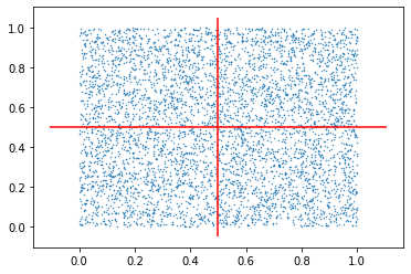
Let us check the number of outcomes falling within the 3rd quadrant. Ideally, they should be 1/4 of the total samples.
jnp.sum(jnp.sum(samples < 0.5, axis=1) == 2)
DeviceArray(1234, dtype=int32)
Sample space: \(\{(x, y)| 0 \le x,y \le 1\}\)
Q: What is an event in Darts game?
A: “all the darts falling within a particular area. For example, in first quadrant.”
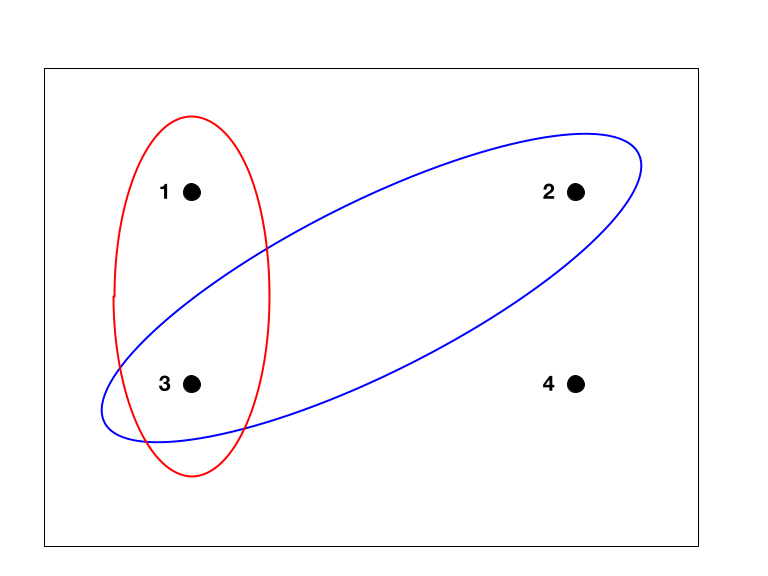
Event in continuos sample space#
In the following image of a continuous space, \(A\) can be considered a event enclosing a particular area.
Probability Axioms#
Recall: Sample space \(\to \Omega\)
\(p(\Omega) = 1\)
\(0 \lt p(event) \le 1\)
If \(A \cap B = \phi\) then \(p(A \cup B) = p(A) + p(B)\)
Questions#
Q: Is \(\Omega\) an event?
A: Yes
Q: What is the probability that you will hit a perticular point on a dart-board?
A: Almost 0. Mathematically, tends to 0.
Q: Consider the following paradox for the dart-board: \(1=P(\Omega)=P(U\{(x, y)\})=\sum P(\{(x, y)\})=\sum 0=0\)
A: Remember Limits!
What is a Random Variable?#
A function that maps our experimental outcome to a numerical value.
Example 1: Coin toss#
key = jax.random.PRNGKey(0)
n_samples = 5

# Sample from the distribution
samples = coin.sample(seed=key, sample_shape=n_samples)
print(samples)
[1 1 1 0 1]
# This function does not work with JAX
# def rv_coin_func(x):
#     if x==1:
#         return 100
#     else:
#         return -20

def rv_coin_func(x):
    return jax.lax.cond(x==1, lambda: 100, lambda: -20)

rv_coin_samples = jax.vmap(rv_coin_func)(samples)
print(rv_coin_samples)
[100 100 100 -20 100]
print(type(samples))
print(type(rv_coin_samples))
<class 'jaxlib.xla_extension.DeviceArray'>
<class 'jaxlib.xla_extension.DeviceArray'>
Example 2: Sum of two dice rolls#
\(X(\omega) = \omega, \text{ where } \omega \text{ can take any value from 1 to 6}\)
\(Y(\omega) = \omega, \text{ where } \omega \text{ can take any value from 1 to 6}\)
\(Z = X + Y\)
\(Z\) can take any value from \(2\) to \(12\).
def Z(sample):
    return jnp.sum(sample)

key = jax.random.PRNGKey(1)
n_samples = 2

# Sample from the distribution
samples = dice.sample(seed=key, sample_shape=n_samples)
rv_samples = jax.vmap(Z)(samples)

print(f"Samples:\n{samples}")
print(f"RV Samples:\n{rv_samples}")
Samples:
[[2 5]
 [5 4]]
RV Samples:
[7 9]
Discrete Random Variables#
Quick Quiz: Is \(C\) a discrete random variable?
A: Yes, because it has countably finite sample space.
Example 1: A student’s score in an exam#
No negative marking.
Sample space = {0, 1, 2, …, 100}
Random variable: \(S(\omega) = \omega, \omega \text{ is marks received}\)
Continuous Random Variables#
Functions defined over a range.
Examples:#
Weights of all human beings on this planet (include past, present and future).
Time taken to blow a baloon by a person.
Programmatic example: Absolute errors#
Experiment: Errors in manufacturing 1000 mm diameter pipes
def abs_rv_func(x):  # RV function
    return jnp.abs(x)

error = distrax.Uniform(low=-10.0, high=10.0)
n_samples = 5

key = jax.random.PRNGKey(0)
samples = error.sample(seed=key, sample_shape=n_samples).round(2)

print(f"Samples: {samples}")
print(f"RV samples: {jax.tree_map(abs_rv_func, samples)}")
Samples: [ 1.49      -8.01      -2.1399999  7.8799996  1.93     ]
RV samples: [1.49      8.01      2.1399999 7.8799996 1.93     ]
Probability Mass Function (for discrete random variables)#
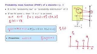
\(p(X=5) = \frac{1}{2}\)
\(p(X=4) = \frac{1}{4}\)
\(p(X=3) = \frac{1}{4}\)
A programmatic example of PMF (for discrete random variables)#
coin = distrax.Bernoulli(probs=0.8)
print(f"Probability of 1: {coin.prob(1):.3f}")
print(f"Probability of 0: {coin.prob(0):.3f}")
Probability of 1: 0.800
Probability of 0: 0.200
print(f"Log probability of 1: {coin.log_prob(1):.3f}")
print(f"Log probability of 0: {coin.log_prob(0):.3f}")
Log probability of 1: -0.223
Log probability of 0: -1.609
Probability Density Function#
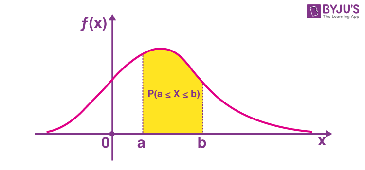
A programmatic example for PDF (for continuous random variables)#
errors = distrax.Uniform(low=1.0, high=2.0)
print(errors.prob(0.5))
0.0
print(errors.prob(1.5))
1.0
print(errors.prob(2.0))
1.0
Summary#
We learned about the following concepts:
Sample space and their types (Discrete and Continuous)
Events
Random Variables and their types (Discrete and Continuous)
How to implement above concepts using
JAXandDistrax