
MLE, MAP and Fully Bayesian (conjugate prior and MCMC) for coin toss
Contents
MLE, MAP and Fully Bayesian (conjugate prior and MCMC) for coin toss#
try:
    import jax
    import jax.numpy as jnp
except:
    ModuleNotFoundError
    %pip install jax jaxlib
    import jax
    import jax.numpy as jnp

try:
    from tensorflow_probability.substrates import jax as tfp
except:
    ModuleNotFoundError
    %pip install tensorflow_probability
    from tensorflow_probability.substrates import jax as tfp

try:
    import daft
except:
    ModuleNotFoundError
    %pip install daft
    import daft

try:
    import optax
except:
    ModuleNotFoundError
    %pip install optax
    import optax

try:
    from rich import print
    from rich.table import Table
except:
    ModuleNotFoundError
    %pip install rich
    from rich import print
    from rich.table import Table


import matplotlib.pyplot as plt
import seaborn as sns
import warnings

warnings.filterwarnings("ignore")
/Users/nipun/miniconda3/lib/python3.8/site-packages/jax/_src/lib/__init__.py:33: UserWarning: JAX on Mac ARM machines is experimental and minimally tested. Please see https://github.com/google/jax/issues/5501 in the event of problems.
  warnings.warn("JAX on Mac ARM machines is experimental and minimally tested. "
dist = tfp.distributions
Creating a dataset#
Let us create a dataset. We will assume the coin toss to be given as per the Bernoulli distribution. We will assume that \(\theta = p(H) = 0.75\) and generate 10 samples. We will fix the random seeds for reproducibility.
We will be encoding Heads as 1 and Tails as 0.
key = jax.random.PRNGKey(0)
WARNING:absl:No GPU/TPU found, falling back to CPU. (Set TF_CPP_MIN_LOG_LEVEL=0 and rerun for more info.)
key
DeviceArray([0, 0], dtype=uint32)
distribution = dist.Bernoulli(probs=0.75)

dataset_100 = distribution.sample(seed=key, sample_shape=(100))
WARNING:root:The use of `check_types` is deprecated and does not have any effect.
dataset_100
DeviceArray([1, 0, 0, 1, 1, 0, 1, 1, 1, 1, 1, 1, 0, 0, 1, 0, 1, 1, 1, 1,
             1, 0, 1, 1, 1, 1, 1, 1, 1, 1, 0, 1, 1, 1, 1, 1, 1, 1, 0, 1,
             1, 1, 1, 0, 0, 0, 1, 1, 1, 0, 1, 1, 0, 1, 1, 1, 1, 0, 1, 1,
             1, 0, 1, 0, 1, 0, 1, 1, 1, 0, 1, 1, 0, 1, 1, 1, 1, 0, 1, 1,
             0, 1, 1, 1, 1, 1, 1, 1, 1, 1, 1, 1, 1, 1, 1, 1, 1, 0, 0, 1],            dtype=int32)
MLE#
Obtaining MLE analytically#
As per the principal of MLE, the best estimate for \(\theta = p(H) = \dfrac{n_h}{n_h+n_t}\)
mle_estimate = dataset_100.sum() / 100
mle_estimate
DeviceArray(0.76, dtype=float32)
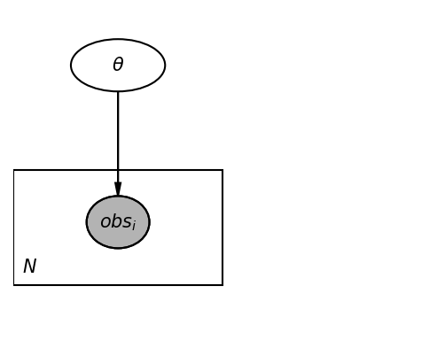
We will now verify if we get the same result using jax+TFP using optimization. But, first, we can create a graphical model for our problem.
pgm = daft.PGM([4, 3], origin=[0, 0])
pgm.add_node(daft.Node("theta", r"$\theta$", 1, 2.5, aspect=1.8))

pgm.add_node(daft.Node("obs", r"$obs_i$", 1, 1, aspect=1.2, observed=True))

pgm.add_edge("theta", "obs")
pgm.add_plate([0, 0.5, 2, 1.0], label=r"$N$", shift=-0.1)
_ = pgm.render(dpi=150)
def neg_log_likelihood(theta, dataset):
    distribution_obj = dist.Bernoulli(probs=theta)
    return -distribution_obj.log_prob(dataset).sum()
We can find the likelihood for different thetas.
neg_log_likelihood(0.2, dataset_100), neg_log_likelihood(0.6, dataset_100)
(DeviceArray(127.67271, dtype=float32), DeviceArray(60.813713, dtype=float32))
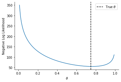
We can also use vmap to compute the likelihood over a range of thetas.
# None for second argument as we don't need vmap for dataset
neg_log_likelihood_vmap = jax.vmap(neg_log_likelihood, in_axes=(0, None))
theta_array = jnp.linspace(0.01, 0.99, 100)
nll_array = neg_log_likelihood_vmap(theta_array, dataset_100)
plt.plot(theta_array, nll_array)
sns.despine()
plt.axvline(0.75, linestyle="--", color="k", label=r"True $\theta$")
plt.legend()
plt.ylabel("Negative Log Likelihood")
_ = plt.xlabel(r"$\theta$")
Learning MLE parameters via gradient descent#
# We need gradient only respect to the first argument
grad_loss = jax.grad(neg_log_likelihood)
grad_loss(0.5, dataset_100)
DeviceArray(-104., dtype=float32, weak_type=True)
grad_loss(0.8, dataset_100)
DeviceArray(25.000008, dtype=float32, weak_type=True)
We can see that the gradient values starting with \(\theta = 0.5\) will push towards increasing \(\theta\) and vice versa starting with \(\theta = 0.8\)
optimizer = optax.sgd(learning_rate=0.001)

theta = jnp.array(0.1).round(2)

opt_state = optimizer.init(theta)
table = Table(title="MLE Convergence")

table.add_column("Iteration", justify="right", style="cyan", no_wrap=True)
table.add_column("Loss", justify="right", style="magenta")
table.add_column("Theta", justify="right", style="green")


for i in range(10):
    cost_val = neg_log_likelihood(theta, dataset_100)
    table.add_row(str(i), f"{cost_val:0.2f}", f"{theta:0.2f}")
    grad_theta_val = grad_loss(theta, dataset_100)
    updates, opt_state = optimizer.update(grad_theta_val, opt_state)
    theta = optax.apply_updates(theta, updates)
print(table)
       MLE Convergence
┏━━━━━━━━━━━┳━━━━━━━━┳━━━━━━━┓
┃ Iteration ┃   Loss ┃ Theta ┃
┡━━━━━━━━━━━╇━━━━━━━━╇━━━━━━━┩
│         0 │ 177.53 │  0.10 │
│         1 │  56.86 │  0.83 │
│         2 │  55.23 │  0.78 │
│         3 │  55.13 │  0.77 │
│         4 │  55.11 │  0.76 │
│         5 │  55.11 │  0.76 │
│         6 │  55.11 │  0.76 │
│         7 │  55.11 │  0.76 │
│         8 │  55.11 │  0.76 │
│         9 │  55.11 │  0.76 │
└───────────┴────────┴───────┘
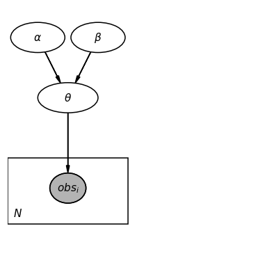
MAP#
pgm = daft.PGM([4, 4], origin=[0, 0])
pgm.add_node(daft.Node("alpha", r"$\alpha$", 0.5, 3.5, aspect=1.8))
pgm.add_node(daft.Node("beta", r"$\beta$", 1.5, 3.5, aspect=1.8))


pgm.add_node(daft.Node("theta", r"$\theta$", 1, 2.5, aspect=2))

pgm.add_node(daft.Node("obs", r"$obs_i$", 1, 1, aspect=1.2, observed=True))

pgm.add_edge("theta", "obs")
pgm.add_edge("alpha", "theta")
pgm.add_edge("beta", "theta")


pgm.add_plate([0, 0.5, 2, 1.0], label=r"$N$", shift=-0.1)
_ = pgm.render(dpi=110)
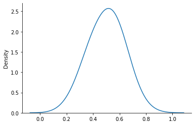
prior_alpha = 10.0
prior_beta = 10.0
prior_dist = dist.Beta(concentration1=prior_alpha, concentration0=prior_beta)
Our prior will give us samples on \(\theta\). Let us draw a 100 samples and draw their histogram.
prior_samples = prior_dist.sample(sample_shape=(100), seed=key)
WARNING:root:The use of `check_types` is deprecated and does not have any effect.
sns.kdeplot(prior_samples, bw_adjust=2)
sns.despine()
Now, given a \(\theta\), we can evaluate the log prior and log likelihood and optimize their sum them to obtain the MAP estimate.
def neg_log_prior(theta, prior_dist):
    return -prior_dist.log_prob(theta)
neg_log_prior(0.1, prior_dist)
DeviceArray(7.9352818, dtype=float32)
neg_log_prior(0.5, prior_dist)
DeviceArray(-1.2595797, dtype=float32)
Clearly, we are much more likely to sample \(\theta = 0.5\) from our prior in comparison to \(\theta = 0.1\).
def joint_neg_log_prior_log_likelihood(theta, dataset, prior_dist):
    return neg_log_prior(theta, prior_dist) + neg_log_likelihood(theta, dataset)
grad_loss = jax.grad(joint_neg_log_prior_log_likelihood)
optimizer = optax.sgd(learning_rate=0.001)

theta = jnp.array(0.1).round(2)

opt_state = optimizer.init(theta)
table = Table(title="MAP Convergence")

table.add_column("Iteration", justify="right", style="cyan", no_wrap=True)
table.add_column("Loss", justify="right", style="magenta")
table.add_column("Theta", justify="right", style="green")


for i in range(10):
    cost_val = joint_neg_log_prior_log_likelihood(theta, dataset_100, prior_dist)
    table.add_row(str(i), f"{cost_val:0.2f}", f"{theta:0.2f}")
    grad_theta_val = grad_loss(theta, dataset_100, prior_dist)
    updates, opt_state = optimizer.update(grad_theta_val, opt_state)
    theta = optax.apply_updates(theta, updates)
print(table)
       MAP Convergence
┏━━━━━━━━━━━┳━━━━━━━━┳━━━━━━━┓
┃ Iteration ┃   Loss ┃ Theta ┃
┡━━━━━━━━━━━╇━━━━━━━━╇━━━━━━━┩
│         0 │ 185.46 │  0.10 │
│         1 │  74.68 │  0.91 │
│         2 │  58.55 │  0.63 │
│         3 │  56.80 │  0.67 │
│         4 │  56.33 │  0.70 │
│         5 │  56.22 │  0.71 │
│         6 │  56.20 │  0.72 │
│         7 │  56.20 │  0.72 │
│         8 │  56.19 │  0.72 │
│         9 │  56.19 │  0.72 │
└───────────┴────────┴───────┘
f"{(dataset_100.sum()+10)/(120):0.2f}"
'0.72'
Analytical Posterior#
\(P(\theta|Data) \sim Beta(\#Heads~in~Data + \alpha, \#Tails~in~Data + \beta)\)
analytical_posterior = dist.Beta(
    dataset_100.sum() + prior_alpha, 100.0 - dataset_100.sum() + prior_beta
)
analytical_posterior.concentration1, analytical_posterior.concentration0
(DeviceArray(86., dtype=float32, weak_type=True),
 DeviceArray(34., dtype=float32, weak_type=True))
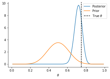
plt.plot(theta_array, analytical_posterior.prob(theta_array), label="Posterior")
plt.plot(theta_array, prior_dist.prob(theta_array), label="Prior")
plt.axvline(0.75, linestyle="--", color="k", label=r"True $\theta$")


sns.despine()
_ = plt.xlabel(r"$\theta$")
plt.legend()
<matplotlib.legend.Legend at 0x1318a1fa0>
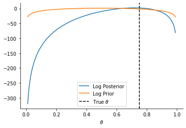
plt.plot(theta_array, analytical_posterior.log_prob(theta_array), label="Log Posterior")
plt.plot(theta_array, prior_dist.log_prob(theta_array), label="Log Prior")
plt.axvline(0.75, linestyle="--", color="k", label=r"True $\theta$")


sns.despine()
_ = plt.xlabel(r"$\theta$")
plt.legend()
<matplotlib.legend.Legend at 0x1319f87c0>
MCMC#
Implementation of Metropolis algorithm from scratch
@jax.jit
def next_sample(cur_sample, key):
    return dist.Normal(loc=cur_sample, scale=0.1, validate_args=False).sample(
        seed=key, sample_shape=()
    )
key = jax.random.PRNGKey(5)
_, k = jax.random.split(key, 2)
next_sample(1.0, k)
WARNING:root:The use of `check_types` is deprecated and does not have any effect.
DeviceArray(1.1064283, dtype=float32)
@jax.jit
def lp(theta):
    return -joint_neg_log_prior_log_likelihood(theta, dataset_100, prior_dist)
lp(0.1)
DeviceArray(-185.46045, dtype=float32)
import numpy as onp
x_start = 0.5
num_iter = 5000
xs = onp.empty(num_iter)
xs[0] = x_start
lu = jnp.log(dist.Uniform(0, 1).sample(sample_shape=[num_iter], seed=k))

keys = jax.random.split(k, num_iter)

for i in range(1, num_iter):
    ns = next_sample(xs[i - 1], keys[i])
    if ns > 0.99:
        ns = 0.99
    if ns < 0.01:
        ns = 0.01
    xs[i] = ns
    la = lp(xs[i]) - lp(xs[i - 1])

    if lu[i] > la:
        xs[i] = xs[i - 1]
WARNING:root:The use of `check_types` is deprecated and does not have any effect.
WARNING:root:The use of `check_types` is deprecated and does not have any effect.
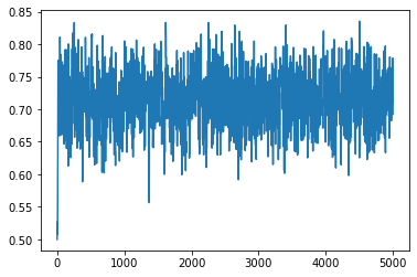
plt.plot(jnp.array(xs).reshape(-1, 1))
[<matplotlib.lines.Line2D at 0x131af5790>]
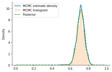
sns.kdeplot(jnp.array(xs), label="MCMC estimate density", lw=2)
plt.hist(onp.array(xs), density=True, label="MCMC histogram", alpha=0.2, bins=10)
plt.plot(
    theta_array,
    analytical_posterior.prob(theta_array),
    label="Posterior",
    lw=2,
    linestyle="--",
)
plt.legend()
sns.despine()
TODO
remove the warnings
check if can replace TFP with distrax here or pure jax.scipy.?
VI from scratch?
Document (and maybe create Class for MH sampling)
Better way for MCMC sampling when parameters are constrained? (like theta between 0 and 1?)
where other can we jit?